Chapter 7 Absorption and Reward

Caveat: From now on, all Markov chains will have finite state spaces.

7.1 Absorption

Remember the “Tennis” example from a few lectures ago and the question we asked there, namely, how does the probability of winning a single point affect the probability of winning the overall game? An algorithm that will help you answer that question will be described in this lecture.

The first step is to understand the structure of the question asked in the light of the canonical decomposition of the previous lecture. In the “Tennis” example, all the states except for the winning ones are transient, and there are two one-element recurrent classes {“Player 1 wins”} and {“Player 2 wins”} The chain starts from a transient state $(0,0)$, moves around a bit, and, eventually, gets absorbed in one of the two. The probability we are interested in is not the probability that the chain will eventually get absorbed. That probability is always $1$. We are, instead, interested in the probability that the absorption will occur in a particular state - the state “Player 1 wins” (as opposed to “Player 2 wins”) in the “Tennis” example.

A more general version of the problem above is the following: let $i\in S$ be any state, and let $j$ be a recurrent state. If the set of all recurrent states is denoted by $C$, and if $\tau_{C}$ is the first hitting time of the set $C$, then $X_{\tau_{C}}$ denotes the first recurrent state visited by the chain. Equivalently, $X_{\tau_{C}}$ is the value of $X$ at (random) time $\tau_{C}$; its value is the name of the state in which it happens to find itself the first time it hits the set of all recurrent states. For any two states $i,j\in S$, the $u_{ij}$ is defined as \[u_{ij}={\mathbb{P}}_i[ X_{\tau_C}=j]={\mathbb{P}}_i[\text{ the first recurrent state visited by $X$ is $j$ }].\] There are several boring situations to discard first:

$j$ is transient: in this case $u_{ij}=0$ for any $i$ because $j$ cannot possibly be the first recurrent state we hit - it is not even recurrent.
$j$ is recurrent, and so is $i$. Since $i$ is recurrent, i.e., $i\in C$, we clearly have $\tau_C=0$. Therefore $u_{ij} = {\mathbb{P}}_i[ X_0= j]$, and this equals to either $1$ or $0$, depending on whether $i=j$ or $i\ne j$.

That leaves us with the situation where $i \in T$ and $j\in C$ as the interesting one. In many calculations related to Markov chains, the method of first-step decomposition works miracles. Simply, we cut the probability space according to what happened in the first step and use the law of total probability (assuming $i\in T$, $j\in C$) \[\label{equ:system-for-u} \nonumber \begin{split} u_{ij} & ={\mathbb{P}}_i[ X_{\tau_C}=j]=\sum_{k\in S} {\mathbb{P}}[X_{\tau_C}=j|X_0=i, X_1=k] {\mathbb{P}}[ X_1=k|X_0=i]\\ &= \sum_{k\in S} {\mathbb{P}}[X_{\tau_C}=j|X_1=k]p_{ik} \end{split}\] The conditional probability ${\mathbb{P}}[X_{\tau_C}=j|X_1=k]$ is an absorption probability, too. If $k=j$, then ${\mathbb{P}}[X_{\tau_C}=j|X_1=k]=1$. If $k\in C\setminus\{j\}$, then we are already in C, but in a state different from $j$, so ${\mathbb{P}}[ X_{\tau_C}=j|X_1=k]=0$. Therefore, the sum above can be written as \[\label{equ:syst} \begin{split} u_{ij}= \sum_{k\in T} p_{ik} u_{kj} + p_{ij}, \end{split}\] which is a system of linear equations for the family $( u_{ij}, i\in T, j\in C)$. Linear systems are typically better understood when represented in the matrix form. Let $U$ be a $T\times C$-matrix $U=(u_{ij}, i\in T, j\in C)$, and let $Q$ be the portion of the transition matrix $P$ corresponding to the transitions from $T$ to $T$, i.e. $Q=(p_{ij},i\in T, j\in T)$, and let $R$ contain all transitions from $T$ to $C$, i.e., $R=(p_{ij})_{i\in T, j\in C}$. If $P_C$ denotes the matrix of all transitions from $C$ to $C$, i.e., $P_C=(p_{ij}, i\in C, j\in C)$, then the canonical form of $P$ looks like this: \[P= \begin{bmatrix} P_C & 0 \\ R & Q \end{bmatrix}.\] The system now becomes: \[U= QU+R,\text{ i.e., } (I-Q) U = R.\] If the matrix $I-Q$ happens to be invertible, we are in business, because we then have an explicit expression for $U$: \[U= (I-Q)^{-1} R.\] So, is $I-Q$ invertible? It is when the state space $S$ is finite; here is the argument, in case you are interested:

Theorem. When the state space $S$ is finite, the matrix $I-Q$ is invertible and \[ \begin{split} (I-Q)^{-1} = \sum_{n=0}^{\infty} Q^n. \end{split}\] Moreover, the entry at the position $i,j$ in $(I-Q)^{-1}$ is the expected total number of visits to the state $j$, for a chain started at $i$.

Proof. For $k\in{\mathbb{N}}$, the matrix $Q^k$ is the same as the submatrix corresponding to the transient states of the full $k$-step transition matrix $P^k$. Indeed, going from a transient state to another transient state in $k$ steps can only happen via other transient states (once we hit a recurrent class, we are stuck there forever).

Using the same idea as in the proof of our recurrence criterion in the previous chapter we can conclude that for any two transient states $i$ and $j$, we have (remember ${\mathbb{E}}_i[ \mathbf{1}_{\{X_n = j\}}] = {\mathbb{P}}_i[X_n = j] = p_{ij}^{(n)}$) \[{\mathbb{E}}_i[ \sum_{n=0}^{\infty} \mathbf{1}_{\{X_n = j\}}] = \sum_{n\in{\mathbb{N}_0}} p^{(n)}_{ij} = \sum_{n\in{\mathbb{N}_0}} q^{(n)}_{ij} = (\sum_{n\in{\mathbb{N}}_0} Q^n)_{ij}.\] On the other hand, the left hand side above is simply the expected number of visits to the state $j$, if we start from $i$. Since both $i$ and $j$ are transient, this number will either be $0$ (if the chain never even reaches $j$ from $i$), or a geometric random variable (if it does). In either case, the expected value of this quantity is finite, and, so \[\sum_{n\in{\mathbb{N}}_0} q^{(n)}_{ij}<\infty.\] Therefore, the matrix sum $F = \sum_{n\in{\mathbb{N}}_0} Q^n$ is well defined, and it remains to make sure that $F = (I-Q)^{-1}$, which follows from the following simple computation: \[QF = Q \sum_{n\in{\mathbb{N}}_0} Q^n = \sum_{n\in{\mathbb{N}}_0} Q^{n+1} = \sum_{n\in{\mathbb{N}}} Q^n = \sum_{n\in{\mathbb{N}}_0} Q^n - I = F - I. \text{ Q.E.D.}\]

When the inverse $(I-Q)^{-1}$ exists (like in the finite case), it is called the fundamental matrix of the Markov chain.

Before we turn to the “Tennis” example, let us analyze a simpler case of Gambler’s ruin with $a=3$.

Problem 7.1 What is the probability that a gambler coming in at $x=\$1$ in a Gambler’s ruin problem with $a=3$ succeeds in “getting rich”? We do not assume that $p=\tfrac{1}{2}$.

Solution. The states $0$ and $3$ are absorbing, and all the others are transient. Therefore $C_1=\{0\}$, $C_2=\{3\}$ and $T=T_1=\{1,2\}$. The transition matrix $P$ in the canonical form (the rows and columns represent the states in the order $0,3,1,2$) \[P= \begin{bmatrix} 1 & 0 & 0 & 0\\ 0 & 1 & 0 & 0\\ 1-p & 0 & 0 & p\\ 0 & p & 1-p & 0 \end{bmatrix}\] Therefore, \[R= \begin{bmatrix} 1-p & 0 \\ 0 & p \end{bmatrix} \text{ and } Q= \begin{bmatrix} 0 & p \\ 1-p & 0 \end{bmatrix}.\] The matrix $I-Q$ is a $2\times 2$ matrix so it is easy to invert: \[(I-Q)^{-1}= \frac{1}{1-p+p^2}\begin{bmatrix} 1 & p \\ 1-p & 1 \end{bmatrix}.\] So \[U= \frac{1}{1-p+p^2}\begin{bmatrix} 1 & p \\ 1-p & 1 \end{bmatrix} \begin{bmatrix} 1-p & 0 \\ 0 & p \end{bmatrix} = \begin{bmatrix} \frac{1-p}{1-p+p^2} & \frac{p^2}{1-p+p^2} \\ \frac{(1-p)^2}{1-p+p^2} & \frac{p}{1-p+p^2} \\ \end{bmatrix}.\] Therefore, for the initial “wealth” is 1, the probability of getting rich before bankruptcy is $u_{13}=p^2/(1-p+p^2)$ (the entry in the first row ($x=1$) and the second column ($a=3$) of $U$.)

Problem 7.2 Find the probability of winning a whole game of Tennis, for a player whose probability of winning a single rally is $p=0.45$.

Solution. In the “Tennis” example, the transition matrix is $20\times 20$, with only 2 recurrent states (each in its own class). In order to find the matrix $U$, we (essentially) need to invert an $18\times 18$ matrix and that is a job for a computer. We start with an R function which produces the transition matrix $P$ as a function of the single-rally probability $p$. Even though we only care about $p=0.45$ here, the extra flexibility will come in handy soon:

S= c("0-0", "0-15", "15-0", "0-30", "15-15", "30-0", "0-40", "15-30", 
     "30-15", "40-0", "15-40", "30-30", "40-15", "40-30", "30-40", 
     "40-40", "40-A", "A-40", "P1", "P2")

tennis_P = function(p) {
  matrix(c( 
    0,1-p,p,0,0,0,0,0,0,0,0,0,0,0,0,0,0,0,0,0,
    0,0,0,1-p,p,0,0,0,0,0,0,0,0,0,0,0,0,0,0,0,
    0,0,0,0,1-p,p,0,0,0,0,0,0,0,0,0,0,0,0,0,0,
    0,0,0,0,0,0,1-p,p,0,0,0,0,0,0,0,0,0,0,0,0,
    0,0,0,0,0,0,0,1-p,p,0,0,0,0,0,0,0,0,0,0,0,
    0,0,0,0,0,0,0,0,1-p,p,0,0,0,0,0,0,0,0,0,0,
    0,0,0,0,0,0,0,0,0,0,p,0,0,0,0,0,0,0,0,1-p,
    0,0,0,0,0,0,0,0,0,0,1-p,p,0,0,0,0,0,0,0,0,
    0,0,0,0,0,0,0,0,0,0,0,1-p,p,0,0,0,0,0,0,0,
    0,0,0,0,0,0,0,0,0,0,0,0,1-p,0,0,0,0,0,p,0,
    0,0,0,0,0,0,0,0,0,0,0,0,0,0,p,0,0,0,0,1-p,
    0,0,0,0,0,0,0,0,0,0,0,0,0,p,1-p,0,0,0,0,0,
    0,0,0,0,0,0,0,0,0,0,0,0,0,1-p,0,0,0,0,p,0,
    0,0,0,0,0,0,0,0,0,0,0,0,0,0,0,1-p,0,0,p,0,
    0,0,0,0,0,0,0,0,0,0,0,0,0,0,0,p,0,0,0,1-p,
    0,0,0,0,0,0,0,0,0,0,0,0,0,0,0,0,1-p,p,0,0,
    0,0,0,0,0,0,0,0,0,0,0,0,0,0,0,p,0,0,0,1-p,
    0,0,0,0,0,0,0,0,0,0,0,0,0,0,0,1-p,0,0,p,0,
    0,0,0,0,0,0,0,0,0,0,0,0,0,0,0,0,0,0,1,0,
    0,0,0,0,0,0,0,0,0,0,0,0,0,0,0,0,0,0,0,1),
 byrow=T, ncol = 20 )
}

The positions of the initial state “0-0” in the state-space vector S is $1$, and the positions of the two absorbing states “P1” and “P2” are $19$ and $20$. Therefore the matrices $Q$ and $R$ are obtained by vector indexing as follows:

P = tennis_P(0.45)
Q = P[1:18, 1:18]
R = P[1:18, 19:20]

Linear systems are solved by using the command solve in R:

I = diag(18)  # the identity matrix the same size as Q
U = solve(I - Q, R)
U[1, ]
## [1] 0.38 0.62

Therefore, the probability that Player 1 wins the entire rally is about $0.377$. Note that this number is smaller than $0.45$, so it appears that the game is designed to make it easier for the better player to win. For more evidence, let’s draw the graph of this probability for several values of $p$ (sapply is the version of apply for vectors):

prob_win = function(p) {
    if (p %in% c(0, 1))
        return(p)
    P = tennis_P(p)
    Q = P[1:18, 1:18]
    R = P[1:18, 19:20]
    U = solve(diag(18) - Q, R)
    U[1, 1]
}
ps = seq(0, 1, by = 0.01)
prob_game = sapply(ps, prob_win)

A graph of p vs. prob_game, where the dashed line is the line $y=x$ looks like this:

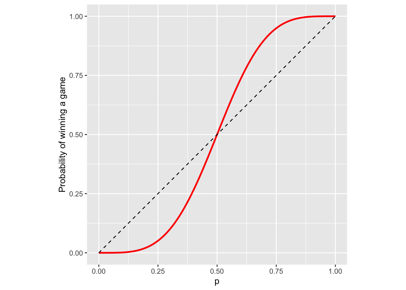
Using a symbolic software package (like Mathematica) we can even get an explicit expression for the win probability in this case: \[\begin{align} u_{(0,0)\ \ "P1\ wins"} = p^4 + 4 p^4 q + 10 p^4 q^2 + \frac{20 p^5 q^3}{1-2pq}. \end{align}\] Actually, you don’t really need computers to derive the expression above. Can you do it by finding all the ways in which the game can be won in $n=4,5,6,8, 10, 12, \dots$ rallies, computing their probabilities, and then adding them all up?

7.2 Expected reward

Suppose that each time you visit a transient state $j\in T$ you receive a reward $g(j)\in{\mathbb{R}}$. The name “reward” is a bit misleading since the negative $g(j)$ corresponds more to a fine than to a reward; it is just a name, anyway. Can we compute the expected total reward before absorption \[v_i={\mathbb{E}}_i[ \sum_{n=0}^{\tau_{C}-1} g(X_n)] ?\] And if we can, what is it good for? Many things, actually, as the following two special cases show:

If $g(j)=1$ for all $j\in T$, then $v_i$ is the expected time until absorption. We will calculate $v_{(0,0)}$ for the “Tennis” example to compute the expected duration of a tennis game.
If $g(k)=1$ and $g(j)=0$ for $j\not =k$, then $v_i$ is the expected number of visits to the state $k$ before absorption. In the “Tennis” example, if $k=(40,40)$, the value of $v_{(0,0)}$ is the expected number of times the score $(40,40)$ is seen in a tennis game.

We compute $v_i$ using the first-step decomposition: \[\label{equ:} % \nonumber \begin{split} v_i &={\mathbb{E}}_i[ \sum_{n=0}^{\tau_C - 1} g(X_n)] = g(i)+ {\mathbb{E}}_i[ \sum_{n=1}^{\tau_C - 1} g(X_n)]\\ &= g(i)+ \sum_{k\in S} {\mathbb{E}}_i[ \sum_{n=1}^{\tau_C - 1} g(X_n)|X_1=k] {\mathbb{P}}_i[X_1=k]\\ & = g(i)+ \sum_{k\in S} p_{ik}{\mathbb{E}}_i[ \sum_{n=1}^{\tau_C - 1} g(X_n)|X_1=k] \end{split}\] If $k\in T$, then the Markov property implies that \[{\mathbb{E}}_i[ \sum_{n=1}^{\tau_C - 1} g(X_n)|X_1=k]={\mathbb{E}}_k[ \sum_{n=0}^{\tau_C - 1} g(X_n)]=v_k.\] When $k\not\in T$, then \[{\mathbb{E}}_i[ \sum_{n=1}^{\tau_C - 1} g(X_n)|X_1=k]=0,\] because we have “arrived” and no more rewards are going to be collected. Therefore, for $i\in T$ we have \[v_i=g(i)+\sum_{k\in T} p_{ik} v_k.\] If we organize all $v_i$ and all $g(i)$ into column vectors $v=(v_i, i\in T)$, $g=(g(i), i\in T)$, we get \[v=Qv+g, \text{ i.e., } v=(I-Q)^{-1} g = Fg.\]

Having derived the general formula for various rewards, we can provide another angle to the interpretation of the fundamental matrix $F$. Let us pick a transient state $j$ and use the reward function $g$ given by \[g(k)=\mathbf{1}_{\{k=j\}}= \begin{cases} 1, & k=j \\ 0,& k\not= j. \end{cases}\] By the discussion above, the $i^{th}$ entry in $v=(I-Q)^{-1} g$ is the expected reward when we start from the state $i$. Given the form of the reward function, $v_i$ is the expected number of visits to the state $j$ when we start from $i$. On the other hand, as the product of the matrix $F=(I-Q)^{-1}$ and the vector $g=(0,0,\dots, 1, \dots, 0)$, $v_i$ is nothing but the $(i,j)$-entry in $F=(I-Q)^{-1}$.

Let’s illustrate these ideas on some of our example chains:

Problem 7.3 What is the expected duration of a game of tennis? Compute it for several values of the parameter $p$.

Solution. The main idea is to perform a reward computation with $g(i)=1$ for all transient states $i$. The R code is very similar to the one in the absorption example:

expected_duration = function(p) {
    if (p %in% c(0, 1))
        return(4)
    P = tennis_P(p)
    Q = P[1:18, 1:18]
    g = matrix(1, nrow = 18, ncol = 1)
    v = solve(diag(18) - Q, g)
    v[1, ]
}
ps = seq(0, 1, by = 0.01)
duration_game = sapply(ps, expected_duration)

As above, here is the graph of p vs. duration_game:

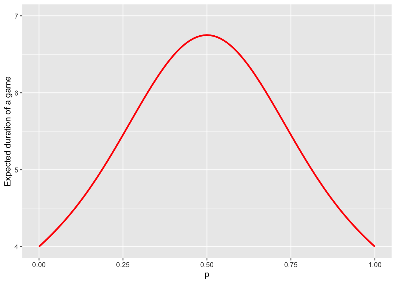
The maximum of the curve about equals to $6.75$, and is achieved when the players are evenly matched ($p=0.5$). Therefore, a game between fairly equally matched opponents lasts $6.75$. The game cannot be shorter than $4$ rallies and that is exactly the expected duration when one player wins with certainty in each rally.

Problem 7.4 What is the expected number of “deuces”, i.e., scores $(40,40)$? Compute it for several values of the parameter $p$.

Solution. This can be computed exactly as above, except that now the reward function is given by \[\begin{align} g(i) = \begin{cases} 1, & \text{ if } i = (40,40),\\ 0, & \text{ otherwise.} \end{cases} \end{align}\] Since the code is almost identical to the code from the last example, we skip it here and only draw the graph: As expected, there are no dueces when $p=0$ or $p=1$, and the maximal expected number of dueces - $0.625$ - occurs when $p=1/2$.

These numbers are a bit misleading, though, and, when asked, people would usually give a higher estimate for this expectation. The reason is that the expectation is a poor summary of for the full distribution of the number of deuces. The best way yo to get a feeling for the entire distribution is to run some simulations. Here is the histogram of $10000$ simulations of a game of tennis for the most interesting case $p=0.5$:

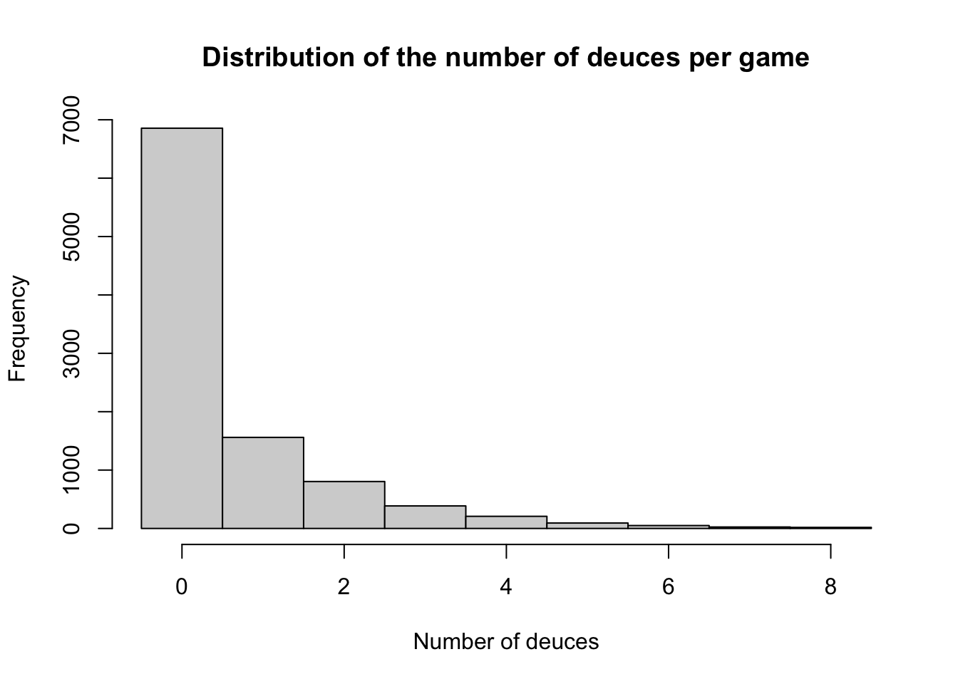
We see that most of the games have no deuces. However, in the cases where a deuce does happen, it is quite possible it will be repeated. A sizable number of draws yielded $4$ of more deuces.

We end with another example from a different area:

Problem 7.5 Alice plays the following game. She picks a pattern consisting of three letters from the set $\{H,T\}$, and then tosses a fair coin until her pattern appears for the first time. If she has to pay $\$1$ for each coin toss, what is the expected cost she is going to incur? What pattern should she choose to minimize that cost?

Solution. We start by choosing a pattern, say $HTH$, and computing the number of coin tosses Alice expects to make before it appears. This is just the kind of computation that can be done using our absorption-and-reward techniques, if we can find a suitable Markov chain. It turns out that the following will do (green arrows stand for probability $1/2$):

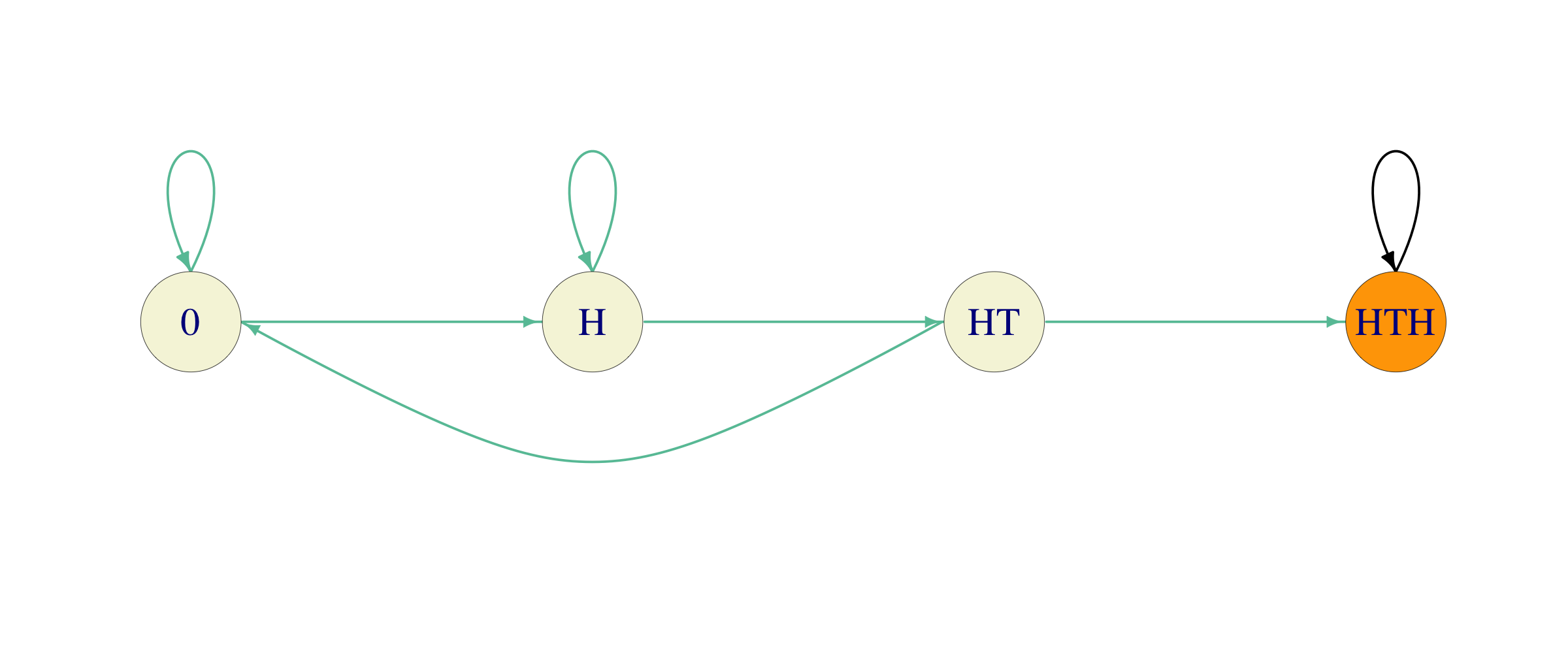
As Alice tosses the coin, she keeps track of the largest initial portion of her pattern that appears at last several places of the sequence of past tosses. The state $0$ represents no such portion (as well as the intial state), while $HT$ means that the last two coin tosses were $H$ and $T$ (in that order) so that it is possible to end the game by tossing a $H$ next. On the other hand, if the last toss was a $T$, there is no need to keep track of that - it is as good as $0$.

Once we have this chain, all we have to do is perform the absorption and reward computation with the reward function $g\equiv 1$. The $Q$-matrix of this chain (with the transient states ordered as $0, H, HT$) is \[Q = \begin{bmatrix} 1/2 & 1/2 & 0 \\ 0 & 1/2 & 1/2 \\ 1/2 & 0 & 0\\ \end{bmatrix}\] and the fundamental matrix $F$ turns out to be \[F = \begin{bmatrix} 4 & 4 & 2 \\ 2 & 4 & 2 \\ 2 & 2 & 2 \\ \end{bmatrix} .\] Therefore, the required expectation is the sum of all the elements on the first row, i.e., $10$.

Let us repeat the same for the pattern $HHH$. We build a similar Markov chain:

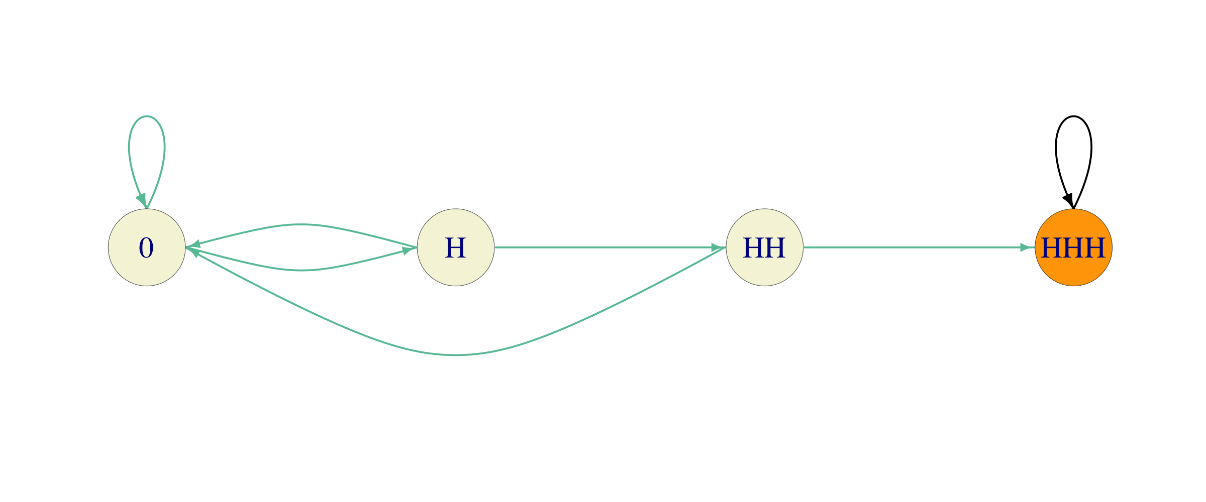
We see that there is a subtle difference. One transition from the state $H$, instead of going back to itself, is directed towards $0$. It is clear from here, that this can only increase Alice’s cost. Indeed, the fundamental matrix is now given by \[F = \begin{bmatrix} 8 & 4 & 2 \\ 6 & 4 & 2 \\ 4 & 2 & 2 \\ \end{bmatrix},\] and the expected number of tosses before the first appearance of $HHH$ comes out as $14$.

Can you do this for other patterns? Which one should Alice choose to minimize her cost?

7.3 Additional Problems for Chapter 7

Note: do not use simulations in any of the problems below. Using R (or other software) to manipulate matrices or perform other numerical computation is fine.

Problem 7.6 The fundamental matrix associated to a finite Markov chain is $F = \begin{bmatrix} 3 & 3 \\ 3/2 & 3\end{bmatrix}$, with the first row (and column) corresponding to the state $A$ and the second to $B$. Some of the following statements are true and the others are false. Find which ones are true and which are false; give explanations for your choices.

The chain has $2$ recurrent states.
If the chain starts in $A$, the expected number of visits to $B$ before hitting the first recurrent state is $3$.
If the chain is equally likely to start from $A$ or $B$, the expected number of steps it will take before it hits its first recurrent state is $\frac{21}{4}$.
${\mathbb{P}}_A[X_1=C] =0$ for any recurrent state $C$.

Click for Solution

Solution.

False. $F$ is $m\times m$, where $m$ is the number of transient states. The dimensions of $F$ say nothing about the number of recurrent states.
True. This is a reward computation with $g = \binom{0}{1}$, so that \[v = Fg = \begin{bmatrix} 3 & 3 \\ 3/2 & 3 \end{bmatrix} \begin{bmatrix} 0 \\ 1 \end{bmatrix} = \begin{bmatrix} 3 \\ 3 \end{bmatrix}.\] Therefore, the expected number of steps is $3$, no matter where we start.
True. Another reward computation, this time with $g=\binom{1}{1}$: \[v = F g = \begin{bmatrix} 6 \\ 9/2\end{bmatrix}.\] Since the two initial states are equally likely, the answer is $\tfrac{1}{2}6 + \tfrac{1}{2}9/2 = \frac{21}{4}$.
True. We know that $F=(I-Q)^{-1}$. Therefore $Q = I -F^{-1}$. We can compute \[F^{-1} = \begin{pmatrix} 2/3 & -2/3 \\ -1/3 & 2/3 \end{pmatrix}.\] This can be done using R or by hand using the formula \[\begin{pmatrix}a & b \\ c & d\end{pmatrix}^{-1}=\frac{1}{ad-bc} \begin{pmatrix} d & -b \\ -c & a\end{pmatrix}.\] Therefore, \[Q = \begin{pmatrix} 1/3 & 2/3 \\ 1/3 & 1/3 \end{pmatrix}\] The first row (transitions from $A$ to transient states) adds up to $1$, so the probability of going from $A$ to any recurrent state in one step must be $0$.

Problem 7.7 In a Markov chain with a finite number of states, the fundamental matrix is given by \[F=\begin{bmatrix} 3 & 4 \\ \tfrac{3}{2} & 4\end{bmatrix}.\] The initial distribution of the chain is uniform on all transient states. Compute the expected value of \[\tau_C=\min \{ n\in{\mathbb{N}}_0\, : \, X_n\in C\},\] where $C$ denotes the set of all recurrent states.

Click for Solution

Solution. Using the reward $g\equiv 1$, the vector $v$ of expected values of $\tau_C$, where each entry corresponds to a different transient initial state is \[v= F g= \begin{bmatrix} 3 & 4 \\ \tfrac{3}{2} & 4\end{bmatrix} \begin{bmatrix} 1 \\ 1 \end{bmatrix} = \begin{bmatrix} 7 \\ \tfrac{11}{2} \end{bmatrix}\] The initial distribution puts equal probabilities on the two transient states, so, by the law of total probability, \[{\mathbb{E}}[\tau_C]= \tfrac{1}{2}\times 7 + \tfrac{1}{2}\times \tfrac{11}{2}= \tfrac{25}{4}.\]

Problem 7.8 Consider the “Gambler’s ruin” model with parameter $p$. Write an R function that computes the (vector of) probabilities that the gambler will go bankrupt before her wealth reaches $\$1000$ for each initial wealth $x = 0,1,\dots, 1000$. Plot the graphs for $p=0.4, p=0.49, p=0.499$ and $p=0.5$ on top of each other. Did you expect them to look the way they do?

Click for Solution

Solution. We use R and start by constructing the matrices $Q$ and $R$ and the solving the system $(I-Q) U = R$.

ruin_probability = function(p) {
    P = matrix(0, ncol = 1001, nrow = 1001)
    P[1, 1] = 1
    P[1001, 1001] = 1
    for (i in 2:1000) {
        P[i, i - 1] = 1 - p
        P[i, i + 1] = p
    }

    Q = P[2:1000, 2:1000]
    R = P[2:1000, c(1, 1001)]
    c(solve(diag(999) - Q, R)[, 1], 0)
}

par(lwd = 2)
plot(ruin_probability(0.4), ylab = "probability of going bankrupt", xlab = "Initial wealth",
    type = "l", col = "maroon", ylim = c(0, 1), lwd = 1)
points(ruin_probability(0.49), type = "l", col = "darkblue", lwd = 1)
points(ruin_probability(0.499), type = "l", col = "seagreen", lwd = 1)
points(ruin_probability(0.5), type = "l", col = "black", lwd = 1)
legend(10, 0.43, legend = c("p=0.5", "p=0.499", "p=0.49", "p=0.4"), col = c("black",
    "seagreen", "darkblue", "maroon"), lty = 1, lwd = 1)

Problem 7.9 A basketball player is shooting a series of free throws. The probability of hitting any single one is $1/2$, and the throws are independent of each other. What is the expected number of throws the player will attempt before hitting 3 free throws in a row (including those 3)?

Click for Solution

Solution. Let $X_n$ be the size of the longest winning streak so far. The value of $X_{n+1}$ then equals $1+X_n$ with probability $1/2$ and $0$ with probability $1/2$ so that the transition matrix of the Markov chain $X$, on the state space $S=\{0,1,2,3\}$ is \[P = \begin{bmatrix} 1/2 & 1/2 & 0 & 0 \\ 1/2 & 0 & 1/2 & 0 \\ 1/2 & 0 & 0 & 1/2 \\ 0 & 0 & 0 & 1\end{bmatrix}\] where we made the state $3$ absorbing. The required expectation is $v_0$, where $v_i$ is the expected number of steps until absorption starting from the state $i$. The system of equations satisfied by $v$ is \[\begin{aligned} v_0 &= 1+ 1/2 v_0 + 1/2 v_1 \\ v_1 &= 1+ 1/2 v_0 + 1/2 v_2 \\ v_2 &= 1+ 1/2 v_0 \end{aligned}\] From here, we get \[\begin{align} v_0 &= 1+ 1/2 v_0 + 1/2 v_1 = 1 + 1/2 v_0 + 1/2 (1+1/2 v_0 + 1/2 v_2)\\ &= 1 + 1/2 v_0 + 1/2 ( 1 + 1/2 v_0 + 1/2(1+1/2 v_0)) \\ &= (1+1/2+1/4) + v_0 (1/2+ 1/4+1/8) = \frac{7}{4} + \frac{7}{8} v_0 \end{align}\] so that $v_0 = 14$.

Problem 7.10 Let $\{X_n\}_{n\in {\mathbb{N}}_0}$ be a Markov chain with the following transition matrix \[P= \begin{bmatrix} 1/2 & 1/2 & 0 \\ 1/3 & 1/3 & 1/3 \\ 0 & 0 & 1\\ \end{bmatrix}\] Suppose that the chain starts from the state $1$.

What is expected time that will pass before the chain first hits $3$?
What is the expected number of visits to state $2$ before $3$ is hit?
Would your answers to 1. and 2. change if we replaced values in the third row of $P$ by any other values (as long as $P$ remains a stochastic matrix)? Would $1$ and $2$ still be transient states?
Use the idea of part 3. to answer the following question. What is the expected number of visits to the state $2$ before a Markov chain with transition matrix \[P= \begin{bmatrix} 17/20 & 1/20 & 1/10\\ 1/15 & 13/15 & 1/15\\ 2/5 & 4/15 & 1/3\\ \end{bmatrix}\] hits the state $3$ for the first time (the initial state is still $1$)? Remember this trick for your next exam.

Click for Solution

Solution. The states 1 and 2 are transient and 3 is recurrent, so the canonical decomposition is $C=\{3\}$, $T=\{1,2\}$ and the canonical form of the transition matrix is \[P= \begin{bmatrix} 1 & 0 & 0 \\ 0 & 1/2 & 1/2 \\ 1/3 & 1/3 & 1/3 \end{bmatrix}\] The matrices $Q$ and $R$ are given by \[Q= \begin{bmatrix} 1/2 & 1/2 \\ 1/3 & 1/3 \end{bmatrix}, R=\begin{bmatrix} 0 \\ 1/3 \end{bmatrix},\] and the fundamental matrix $F=(I-Q)^{-1}$ is \[F= \begin{bmatrix} 4 & 3 \\ 2 & 3 \end{bmatrix}.\]

The reward function $g(1)=g(2)=1$, i.e. $g= \begin{bmatrix} 1 \\ 1 \end{bmatrix}$ will give us the expected time until absorption: \[v=Fg= \begin{bmatrix} 4 & 3 \\ 2 & 3 \end{bmatrix} \begin{bmatrix} 1 \\ 1 \end{bmatrix}= \begin{bmatrix} 7 \\ 5 \end{bmatrix}.\] Since the initial state is $i=1$, the expected time before we first hit $3$ is $v_1=7$.
Here we use the reward function \[g(i)= \begin{cases} 0, & i=1,\\ 1, & i=2. \end{cases}\] to get \[v=Fg= \begin{bmatrix} 4 & 3 \\ 2 & 3 \end{bmatrix} \begin{bmatrix} 0 \\ 1 \end{bmatrix}= \begin{bmatrix} 3 \\ 3 \end{bmatrix},\] so the answer is $v_1=3$.
No, they would not. Indeed, these numbers only affect what the chain does after it hits $3$ for the first time, and that is irrelevant for calculations about the events which happen prior to that.

No, all states would be recurrent. The moral of the story that the absorption calculations can be used even in the settings where all states are recurrent. You simply need to adjust the probabilities, as shown in the following part of the problem.
We make the state $3$ absorbing (and states $1$ and $2$ transient) by replacing the transition matrix by the following one: \[P= \begin{bmatrix} 17/20 & 1/20 & 1/10\\ 1/15 & 13/15 & 1/15\\ 0 & 0 & 1\\ \end{bmatrix}\] The new chain behaves exactly like the old one until it hits $3$ for the first time. Now we find the canonical decomposition and compute the matrix $F$ as above and get \[F=\begin{bmatrix}8 & 3 \\ 4 & 9\end{bmatrix},\] so that the expected number of visits to $2$ (with initial state $1$) is $F_{12}=3$.

Problem 7.11 A fair 6-sided die is rolled repeatedly, and for $n\in{\mathbb{N}}$, the outcome of the $n$-th roll is denoted by $Y_n$ (it is assumed that $\{Y_n\}_{n\in{\mathbb{N}}}$ are independent of each other). For $n\in{\mathbb{N}}_0$, let $X_n$ be the remainder (taken in the set $\{0,1,2,3,4\}$) left after the sum $\sum_{k=1}^n Y_k$ is divided by $5$, i.e. $X_0=0$, and \[%\label{} \nonumber \begin{split} X_n= \sum_{k=1}^n Y_k \ (\,\mathrm{mod}\, 5\,),\text{ for } n\in{\mathbb{N}}, \end{split}\] making $\{X_n\}_{n\in {\mathbb{N}}_0}$ a Markov chain on the state space $\{0,1,2,3,4\}$ (no need to prove this fact).

Write down the transition matrix of the chain.
Classify the states, separate recurrent from transient ones, and compute the period of each state.
Compute the expected number of rolls before the first time $\{X_n\}_{n\in {\mathbb{N}}_0}$ visits the state $2$, i.e., compute ${\mathbb{E}}[\tau_2]$, where \[\tau_2=\min \{ n\in{\mathbb{N}}_0\, : \, X_n=2\}.\]
Compute ${\mathbb{E}}[\sum_{k=0}^{\tau_2-1} X_k]$.

Click for Solution

Solution.

The outcomes $1,2,3,4,5,6$ leave remainders $1,2,3,4,0,1$, when divided by $5$, so the transition matrix $P$ of the chain is given by \[P=\begin{bmatrix} \frac{1}{6} & \frac{1}{3} & \frac{1}{6} & \frac{1}{6} & \frac{1}{6} \\ \frac{1}{6} & \frac{1}{6} & \frac{1}{3} & \frac{1}{6} & \frac{1}{6} \\ \frac{1}{6} & \frac{1}{6} & \frac{1}{6} & \frac{1}{3} & \frac{1}{6} \\ \frac{1}{6} & \frac{1}{6} & \frac{1}{6} & \frac{1}{6} & \frac{1}{3} \\ \frac{1}{3} & \frac{1}{6} & \frac{1}{6} & \frac{1}{6} & \frac{1}{6} \\ \end{bmatrix}\]
Since $p_{ij}>0$ for all $i,j\in{\mathcal{S}}$, all the states belong to the same class, and, because there is at least one recurrent state in a finite-state-space Markov chain and because recurrence is a class property, all states are recurrent. Finally, $1$ is in the return set of every state, so the period of each state is $1$.
In order to be able to use “absorption-and-reward” computations, we turn the state $2$ into an absorbing state, i.e., modify the transition matrix as follows \[P'=\begin{bmatrix} \frac{1}{6} & \frac{1}{3} & \frac{1}{6} & \frac{1}{6} & \frac{1}{6} \\ \frac{1}{6} & \frac{1}{6} & \frac{1}{3} & \frac{1}{6} & \frac{1}{6} \\ 0 & 0 & 1 & 0 & 0 \\ \frac{1}{6} & \frac{1}{6} & \frac{1}{6} & \frac{1}{6} & \frac{1}{3} \\ \frac{1}{3} & \frac{1}{6} & \frac{1}{6} & \frac{1}{6} & \frac{1}{6} \\ \end{bmatrix}\] Now, the first hitting time of the state $2$ corresponds exactly to the absorption time, i.e., the time $\tau_C$ the chain hits its first recurrent state (note that for the new transition probabilities the state $2$ is recurrent and all the other states are transient). In the canonical form, the new transition matrix looks like \[\begin{bmatrix} 1 & 0 & 0 & 0 & 0 \\ \frac{1}{6} & \frac{1}{6} & \frac{1}{3} & \frac{1}{6} & \frac{1}{6} \\ \frac{1}{3} & \frac{1}{6} & \frac{1}{6} & \frac{1}{6} & \frac{1}{6} \\ \frac{1}{6} & \frac{1}{6} & \frac{1}{6} & \frac{1}{6} & \frac{1}{3} \\ \frac{1}{6} & \frac{1}{3} & \frac{1}{6} & \frac{1}{6} & \frac{1}{6} \\ \end{bmatrix}\] Therefore, \[Q= \begin{bmatrix} \frac{1}{6} & \frac{1}{3} & \frac{1}{6} & \frac{1}{6} \\ \frac{1}{6} & \frac{1}{6} & \frac{1}{6} & \frac{1}{6} \\ \frac{1}{6} & \frac{1}{6} & \frac{1}{6} & \frac{1}{3} \\ \frac{1}{3} & \frac{1}{6} & \frac{1}{6} & \frac{1}{6} \\ \end{bmatrix}.\] The expected time until absorption is given by an “absorption-and-reward” computation with the reward matrix \[g_1= \begin{bmatrix} 1 \\ 1 \\ 1 \\ 1 \end{bmatrix}\]

Q = 1/6*matrix(
  c(1,2,1,1,
    1,1,1,1,
    1,1,1,2,
    2,1,1,1), 
  byrow=T, ncol=4)
g1 = matrix(1, nrow=4, ncol=1)
(v = solve( diag(4) - Q, g1 ))
##      [,1]
## [1,]  4.9
## [2,]  4.2
## [3,]  5.0
## [4,]  5.0

Since we are starting from state $1$, the answer is 4.86.

This is an “absorption-and-reward” computation with reward $g_2$ given by \[g_2= \begin{bmatrix} 0 \\ 1 \\ 3 \\ 4 \end{bmatrix}\]

g2 = matrix(c(0, 1, 3, 4), nrow = 4, ncol = 1)
(v = solve(diag(4) - Q, g2))
##      [,1]
## [1,]  7.4
## [2,]  7.2
## [3,] 11.1
## [4,] 11.4

so that ${\mathbb{E}}[\sum_{k=0}^{\tau_2-1} X_k]=$ 7.35.

Problem 7.12 Let $\{Y_n\}_{n\in {\mathbb{N}}_0}$ be a sequence of die-rolls, i.e., a sequence of independent random variables with distribution \[Y_n \sim \left( \begin{array}{cccccc} 1 & 2 & 3 & 4 & 5 & 6 \\ 1/6 & 1/6 & 1/6 & 1/6 & 1/6 & 1/6 \end{array} \right).\] Let $\{X_n\}_{n\in {\mathbb{N}}_0}$ be a stochastic process defined by $X_n=\max (Y_0,Y_1, \dots, Y_n)$. In words, $X_n$ is the maximal value rolled so far.

Explain why $X$ is a Markov chain, and find its transition matrix and the initial distribution.
Supposing that the first roll of the die was $3$, i.e., $X_0=3$, what is the expected time until a $6$ is reached?
Under the same assumption as above ($X_0=3$), what is the probability that a $5$ will not be rolled before a $6$ is rolled for the first time?
Starting with the first value $X_0=3$, each time a die is rolled, the current record (the value of $X_n$) is written down. When a $6$ is rolled for the first time all the numbers are added up and the result is called $S$ (the final $6$ is not counted). What is the expected value of $S$?

Click for Solution

Solution.

The value of $X_{n+1}$ is either going to be equal to $X_n$ if $Y_{n+1}$ happens to be less than or equal to it, or it moves up to $Y_{n+1}$, otherwise, i.e., $X_{n+1}=\max(X_n,Y_{n+1})$. Therefore, the distribution of $X_{n+1}$ depends on the previous values $X_0,X_1,\dots, X_n$ only through $X_n$, and, so, $\{X_n\}_{n\in {\mathbb{N}}_0}$ is a Markov chain on the state space $S=\{1,2,3,4,5,6\}$. The transition Matrix is given by \[P=\begin{bmatrix} 1/6 & 1/6 & 1/6 & 1/6 & 1/6 & 1/6 \\ 0 & 1/3 & 1/6 & 1/6 & 1/6 & 1/6 \\ 0 & 0 & 1/2 & 1/6 & 1/6 & 1/6 \\ 0 & 0 & 0 & 2/3 & 1/6 & 1/6 \\ 0 & 0 & 0 & 0 & 5/6 & 1/6 \\ 0 & 0 & 0 & 0 & 0 & 1/6 \\ \end{bmatrix}\]
We can restrict our attention to the Markov chain on the state space $S=\{3,4,5,6\}$ with the transition matrix \[P=\begin{bmatrix} 1/2 & 1/6 & 1/6 & 1/6 \\ 0 & 2/3 & 1/6 & 1/6 \\ 0 & 0 & 5/6 & 1/6 \\ 0 & 0 & 0 & 1/6 \\ \end{bmatrix}\] The state $6$ is absorbing (and therefore recurrent), while all the others are transient, so the canonical form of the matrix (with the canonical decomposition $C=\{6\}$, $T=\{3,4,5\}$ is given by \[\begin{bmatrix} 1 & 0 & 0 & 0 \\ 1/6 & 1/2 & 1/6 & 1/6 \\ 1/6 & 0 & 2/3 & 1/6 \\ 1/6 & 0 & 0 & 5/6 \\ \end{bmatrix}\] The fundamental matrix $F=(I-Q)^{-1}$ is now given by \[F= \begin{bmatrix} 1/2 & - 1/6 & - 1/6 \\ 0 & 1/3 & - 1/6 \\ 0 & 0 & 1/6\end{bmatrix}^{-1}= \begin{bmatrix} 2 & 1 & 3 \\ 0 & 3 & 3 \\ 0 & 0 & 6 \end{bmatrix}\] The expected time to absorption can be computed by using the reward $1$ for each state: \[F \begin{bmatrix}1 \\ 1 \\ 1\end{bmatrix}= \begin{bmatrix}6\\ 6\\ 6\end{bmatrix}\] Therefore it will take on average 6 rolls until the first $6$.

Note: You don’t need Markov chains to solve this part; the expected time to absorption is nothing but the waiting time until the first $6$ is rolled - a shifted geometrically distributed random variable with parameter $1/6$. Therefore, its expectation is $1+ \frac{5/6}{1/6}=6$.
We make the state $5$ absorbing and the canonical decomposition changes to $C=\{5\}$, $T=\{3,4,6\}$. The canonical form of the transition matrix is \[\begin{bmatrix} 1 & 0 & 0 & 0 \\ 0 & 1 & 0 & 0 \\ 1/6 & 1/6 & 1/2 & 1/6 \\ 1/6 & 1/6 & 0 & 2/3 \\ \end{bmatrix}\] and so \[Q=\begin{bmatrix} 1/2 & 1/6 \\ 0 & 2/3 \end{bmatrix}\text{ and } R=\begin{bmatrix}1/6 & 1/6 \\ 1/6 & 1/6\end{bmatrix}.\] Therefore, the absorption probabilities are the entries of the matrix \[(I-Q)^{-1} R = \begin{bmatrix} 1/2 & 1/2 \\ 1/2 & 1/2\end{bmatrix},\] and the answer is $1/2$.

Note: You don’t need Markov chains to solve this part either; the probability that $6$ will be seen before $5$ is the same as the probability that $5$ will appear before $6$. The situation is entirely symmetric. Therefore, the answer must be $1/2$.
This problem is about expected reward, where the reward $g(i)$ of the state $i\in\{3,4,5\}$ is $g(i)=i$. The answer is $v_3$, where \[v= F \begin{bmatrix}3 \\ 4 \\ 5\end{bmatrix}= \begin{bmatrix}25 \\ 27 \\30\end{bmatrix},\] i.e., the expected value of the sum is $25$.

Note: Can you do this without the use of the Markov-chain theory?

Problem 7.13 Go back to the problem with Basil the rat in the he first lecture on Markov chains and answer the question 2., but this time using an absorption/reward computation.

Click for Solution

Solution. We reuse the Markov chain constructed in the original problem:

P = matrix(0,nrow =7, ncol=7 )
P[1,2] = 1/2; P[1,3] = 1/2;
P[2,1] = 1/3; P[2,4] = 1/3; P[2,6] = 1/3;
P[3,1] = 1/3; P[3,4] = 1/3; P[3,7] = 1/3;
P[4,2] = 1/3; P[4,3] = 1/3; P[4,5] = 1/3;
P[5,4] = 1/2; P[5,6] = 1/2;
P[6,6] = 1
P[7,7] = 1

The states $6$ and $7$ are absorbing, and we can rephrase our problem as follows: what is the probability that the first recurrent state the chain visits is “6”. To answer it, we perform an absorption computation ($3$ and $2$ are the positions of the initial state state “Shock” among transient and recurrent states, respectively)

Q = P[1:5, 1:5]
R = P[1:5, 6:7]
U = solve(diag(5) - Q, R)
(U[3, 2])
## [1] 0.58

Problem 7.14 Go back to the problem with the professor and his umbrellas in the first lecture on Markov chains and answer the questions in part 2., but this time using an absorption/reward computation.

Click for Solution

Solution. We reuse the Markov chain constructed in the original problem:

S= c("h0-4", "h1-3", "h2-2", "h3-1", "h4-0", 
     "0-4o", "1-3o", "2-2o", "3-1o", "4-0o", "Wet")

P = matrix(c( 
  0, 0, 0, 0, 0, 0.95, 0, 0, 0, 0, 0.05,  
  0, 0, 0, 0, 0, 0.05, 0.95, 0, 0, 0, 0,  
  0, 0, 0, 0, 0, 0, 0.05, 0.95, 0, 0, 0,  
  0, 0, 0, 0, 0, 0, 0, 0.05, 0.95, 0, 0,  
  0, 0, 0, 0, 0, 0, 0, 0, 0.05, 0.95, 0,  
  0.8, 0.2, 0, 0, 0, 0, 0, 0, 0, 0, 0,  
  0, 0.8, 0.2, 0, 0, 0, 0, 0, 0, 0, 0,  
  0, 0, 0.8, 0.2, 0, 0, 0, 0, 0, 0, 0,  
  0, 0, 0, 0.8, 0.2, 0, 0, 0, 0, 0, 0,  
  0, 0, 0, 0, 0.8, 0, 0, 0, 0, 0, 0.2,  
  0, 0, 0, 0, 0, 0, 0, 0, 0, 0, 1 ),
 byrow=T, ncol = 11 )

The only absorbing state is “Wet”, so the matrices $Q$ and $R$ are easy to define as sub-matrices of $P$:

Q = P[1:10, 1:10]
R = P[1:10, 11]

The expected number of trips can be obtained using a reward computation with $g=1$:

g = matrix(1, nrow = 10, ncol = 1)
v = solve(diag(10) - Q, g)
(v[3, ])  # 3 is the number of the initial state 'h2-2'
## [1] 39

The expected number of days before the professor gets wet is half of that, i.e. 19.57.

For the second question, we need to add another state to the chain, i.e. split the state “Wet” into two states “Wet-h” and “Wet-o” in order to keep track of the last location professor left before he got wet.

S= c("h0-4", "h1-3", "h2-2", "h3-1", "h4-0", "0-4o", 
     "1-3o", "2-2o", "3-1o", "4-0o", "Wet-o", "Wet-h")
 
P = matrix(c( 
  0, 0, 0, 0, 0, 0.95, 0, 0, 0, 0, 0, 0.05,  
  0, 0, 0, 0, 0, 0.05, 0.95, 0, 0, 0, 0, 0,  
  0, 0, 0, 0, 0, 0, 0.05, 0.95, 0, 0, 0, 0,  
  0, 0, 0, 0, 0, 0, 0, 0.05, 0.95, 0, 0, 0,  
  0, 0, 0, 0, 0, 0, 0, 0, 0.05, 0.95, 0, 0,  
  0.8, 0.2, 0, 0, 0, 0, 0, 0, 0, 0, 0, 0,  
  0, 0.8, 0.2, 0, 0, 0, 0, 0, 0, 0, 0, 0,  
  0, 0, 0.8, 0.2, 0, 0, 0, 0, 0, 0, 0, 0,  
  0, 0, 0, 0.8, 0.2, 0, 0, 0, 0, 0, 0, 0,  
  0, 0, 0, 0, 0.8, 0, 0, 0, 0, 0, 0.2, 0,  
  0, 0, 0, 0, 0, 0, 0, 0, 0, 0, 1, 0,  
  0, 0, 0, 0, 0, 0, 0, 0, 0, 0, 0, 1 ),
 byrow=T, ncol = 12 )

The question can now be rephrased as follows: what is the probability that the first recurrent state the chain visits is “Wet-o”. To answer it, we perform an absorption computation ($3$ and $1$ are the positions of the initial state “h2-2” and the state “Wet-o” among transient and recurrent states, respectively)

Q = P[1:10, 1:10]
R = P[1:10, 11:12]
U = solve(diag(10) - Q, R)
(U[3, 1])
## [1] 0.99

Problem 7.15 An airline reservation system has two computers. Any computer in operation may break down on any given day with probability $p=0.3$, independently of the other computer. There is a single repair facility which takes two days to restore a computer to normal. It can work on only one computer at a time, and if two computers need work at the same time, one of them has to wait and enters the facility as soon as it is free again.

The system starts with one operational computer; the other one broke last night and just entered the repair facility this morning.

Compute the probability that at no time will both computers be down simultaneously between now and the first time both computers are operational.
Assuming that each day with only one working computer costs the company $\$10,000$ and each day with both computers down $\$30,000$, what is the total cost the company is expected to incur between now and the first time both computers are operational again.

Click for Solution

Solution. Any of the computers can be in one of the following 4 conditions: in operation (OK), in repair facility - 2nd day (R2), in repair facility - 1st day (R1), waiting to enter the repair facility (W). Since there are two computers, each state of the Markov chain will be a quadruple of numbers $(OK, R2, R1, W)$ denoting the number of computers in each conditions. For example, 1-0-1-0 means that there is one computer in operation (OK) and one which is spending its first day in the repair facility (R1). If there are no computers in operation, the chain moves deterministically, but if 1 or 2 computers are in operation, they break down with probability p each, independently of the other. For example, if there are two computers in operation (the state of the system being 2-0-0-0), there are 3 possible scenarios: both computers remain in operation (that happens with probability $(1 − p)^2$), exactly one computer breaks down (the probability of that is $2p(1 − p)$) and both computers break down (with probability $p^2$). In the first case, the chain stays in the state 2-0-0-0. In the second case, the chain moves to the state 1-0-1-0 and in the third case one of the computers enters the repair facility, while the other spends a day waiting, which corresponds to the state 1-0-1-0. All in all, here is the transition graph of the chain:

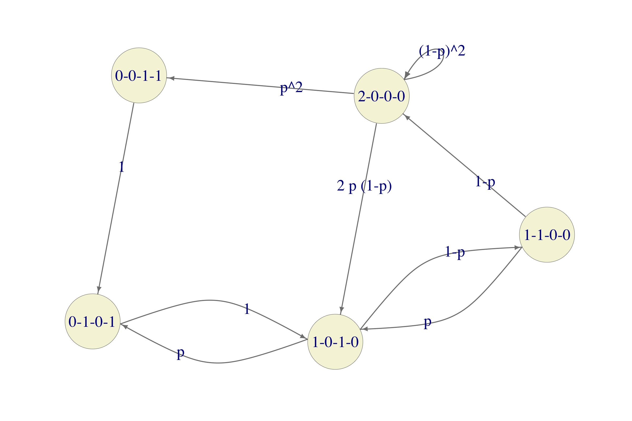
In this problem we only care about what happens after both computers are operational again, we might as well make the state 2-0-0-0 an absorbing state and remove the existing transitions from 2-0-0-0 to other states. The state 0-0-1-1 can also be removed because there is no way to get there from the initial state 1-0-1-0 without passing through 2-0-0-0 which we just “blocked”. The simplified chain will therefore look like this:

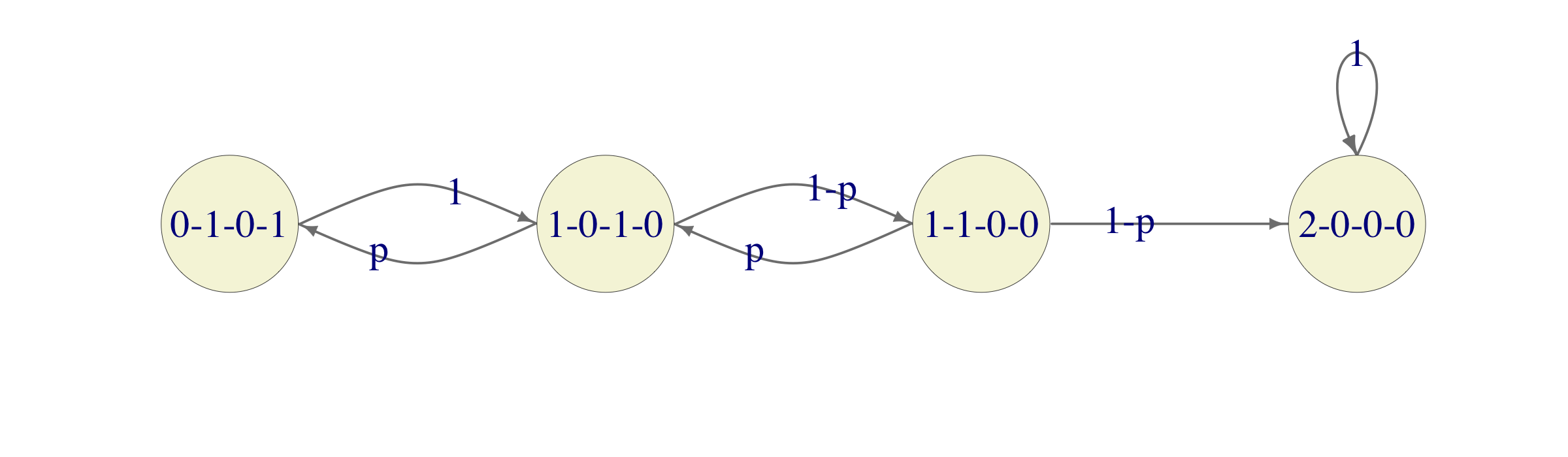
To interpret this as an absorption question, we need to simplify our chain a bit more and turn 0-1-0-1 into an absorbing state. This way, we get the following chain

The lucky break is that this is a Gambler’s-ruin chain with $a=3$, the probability of winning $1-p$ and the initial wealth $1$. According to the worked-out Example in the notes this probability is given by $(1-p)^2/(p+(1-p)^2)$ (remember, our probability of winning is $1-p$, and not $p$), which, for $p=0.3$ evaluates to about $0.62$
This is a reward-type question for the original (simplified) chain. Unfortunately, this is not a Gambler’s-ruin chain, so we will have to perform all the computations in this case. This chain has 3 transient and one recurrent (absorbing) state and the reward (cost) of visiting state 0-1-0-1 is $30,000$ and $10,000$ for states 1-0-1-0 and 1-1-0-0. The entire computation is performed in the chunk below:

p = 0.3
Tr = c("0-1-0-1", "1-0-1-0", "1-1-0-0")
Q = matrix(c(0, 1, 0, p, 0, 1 - p, 0, p, 0), nrow = 3, ncol = 3, byrow = TRUE)
g = matrix(c(30000, 10000, 10000), nrow = 3)
solve(diag(3) - Q, g)[2, 1]  #The initial state is 2 (1-0-1-0)
## [1] 53061