Chapter 3 Random Walks

3.1 What are stochastic processes?

A stochastic process is a sequence - finite or infinite - of random variables. We usually write \(\{X_n\}_{n\in{\mathbb{N}}_0}\) or \(\{X_n\}_{0\leq n \leq T}\), depending on whether we are talking about an infinite or a finite sequence. The number \(T\in {\mathbb{N}}_0\) is called the time horizon, and we sometimes set \(T=+\infty\) when the sequence is infinite. The index \(n\) is often interpreted as time, so that a stochastic process can be thought of as a model of a random process evolving in time. The initial value of the index \(n\) is often normalized to \(0\), even though other values may be used. This it usually very clear from the context.

It is important that all the random variables \(X_0, X_1,\dots\) “live” on the same sample space \(\Omega\). This way, we can talk about the notion of a trajectory or a sample path of a stochastic process: it is, simply, the sequence of numbers \[X_0(\omega), X_1(\omega), \dots\] but with \(\omega\in \Omega\) considered “fixed”. In other words, we can think of a stochastic process as a random variable whose value is not a number, but sequence of numbers. This will become much clearer once we introduce enough examples.

3.2 The Simple Symmetric Random Walk

A stochastic process \(\{X\}_{n\in{\mathbb{N}}_0}\) is said to be a simple symmetric random walk (SSRW) if

\(X_0=0\),
the random variables \(\delta_1 = X_1-X_0\), \(\delta_2 = X_2 - X_1\), …, called the steps of the random walk, are independent
each \(\delta_n\) has a coin-toss distribution, i.e., its distribution is given by \[{\mathbb{P}}[ \delta_n = 1] = {\mathbb{P}}[ \delta_n=-1] = \tfrac{1}{2} \text{ for each } n.\]

Some comments:

This definition captures the main features of an idealized notion of a particle that gets shoved, randomly, in one of two possible directions, over and over. In other words, these “shoves” force the particle to take a step, and steps are modeled by the random variables variables \(\delta_1,\delta_2, \dots\). The position of the particle after \(n\) steps is \(X_n\); indeed, \[X_n = \delta_1 + \delta_2 + \dots + \delta_n \text{ for }n\in {\mathbb{N}}.\] It is important to assume that any two steps are independent of each other - the most important properties of random walks depend on this in a critical way.
Sometimes, we only need a finite number of steps of a random walk, so we only care about the random variables \(X_0, X_1,\dots, X_T\). This stochastic process (now with a finite time horizon \(T\)) will also be called a random walk. If we want to stress that the horizon is not infinite, we sometimes call it the finite-horizon random walk. Whether \(T\) is finite or infinite is usually clear from the context.
The starting point \(X_0=0\) is just a normalization. Sometimes we need more flexibility and allow our process to start at \(X_0=x\) for some \(x\in {\mathbb{N}}\). To stress that fact, we talk about the random walk starting at \(x\). If no starting point is mentioned, you should assume \(X_0=0\).
We will talk about biased (or asymmetric) random walks a bit later. The only difference will be that the probabilities of each \(\delta_n\) taking values \(1\) or \(-1\) will be \(p\in (0,1)\) and \(1-p\), and not necessarily \(\tfrac{1}{2}\), The probability \(p\) cannot change from step to step and the steps \(\delta_1, \delta_2, \dots\) will continue to be independent from each other.
The word simple in its name refers to the fact that distribution of every step is a coin toss. You can easily imagine a more complicated mechanism that would govern each step. For example, not only the direction, but also the size of the step could be random. In fact, any distribution you can think of can be used as a step distribution of a random walk. Unfortunately, we will have very little to say about such, general, random walks in these notes.

3.3 How to simulate random walks

In addition to being quite simple conceptually, random walks are also easy to simulate. The fact that the steps \(\delta_n = X_n - X_{n-1}\) are independent coin tosses immediately suggests a feasible strategy: simulate \(T\) independent coin tosses first, and then define each \(X_n\) as the sum of the first \(n\) tosses.

Before we implement this idea in R, let us agree on a few conventions which we will use whenever we simulate a stochastic process:

the result of each simulation is a data.frame object
its columns will be the random variables \(X_0\), \(X_1\), It is a good idea to name your columns X0, X1, X2, etc.
each row will represent one “draw”:

This is best achieved by the following two-stage approach in R:

write a function which will simulate a single trajectory of your process, If your process comes with parameters, it is a good idea to include them as arguments to this function.
use the function replicate to stack together many such simulations and convert the result to a data.frame. Don’t forget to transpose after (use the function t) because replicate works column by column, and not row by row.

Let’s implement this in the case of a simple random walk. Of course, it is impossible to simulate a random walk on an infinite horizon (\(T=\infty\)) so we must restrict to finite-horizon random walks⁶. The function cumsum which produces partial sums of its input comes in very handy.

single_trajectory = function(T, p = 0.5) {
    delta = sample(c(-1, 1), size = T, replace = TRUE, prob = c(1 - p, p))
    x = cumsum(delta)
    return(x)
}

Next, we run the same function nsim times and record the results. It is a lucky break that the default names given to columns are X1, X2, … so we don’t have to rename them. We do have to add the zero-th column \(X_0=0\) because, formally speaking, the “random variable” \(X_0=0\) is a part of the stochastic process. This needs to be done before other columns are added to maintain the proper order of columns, which is important when you want to plot trajectories.

simulate_walk = function(nsim, T, p = 0.5) {
  return(
    data.frame(
      X0 = 0,
      t(replicate(nsim, single_trajectory(T, p)))
    ))
}
walk = simulate_walk(nsim = 10000, T = 500)

3.4 Two ways of looking at a stochastic proceses

Now that we have the data frame walk, we can explore in at least two qualitatively different ways:

3.4.1 Column-wise (distributionally)

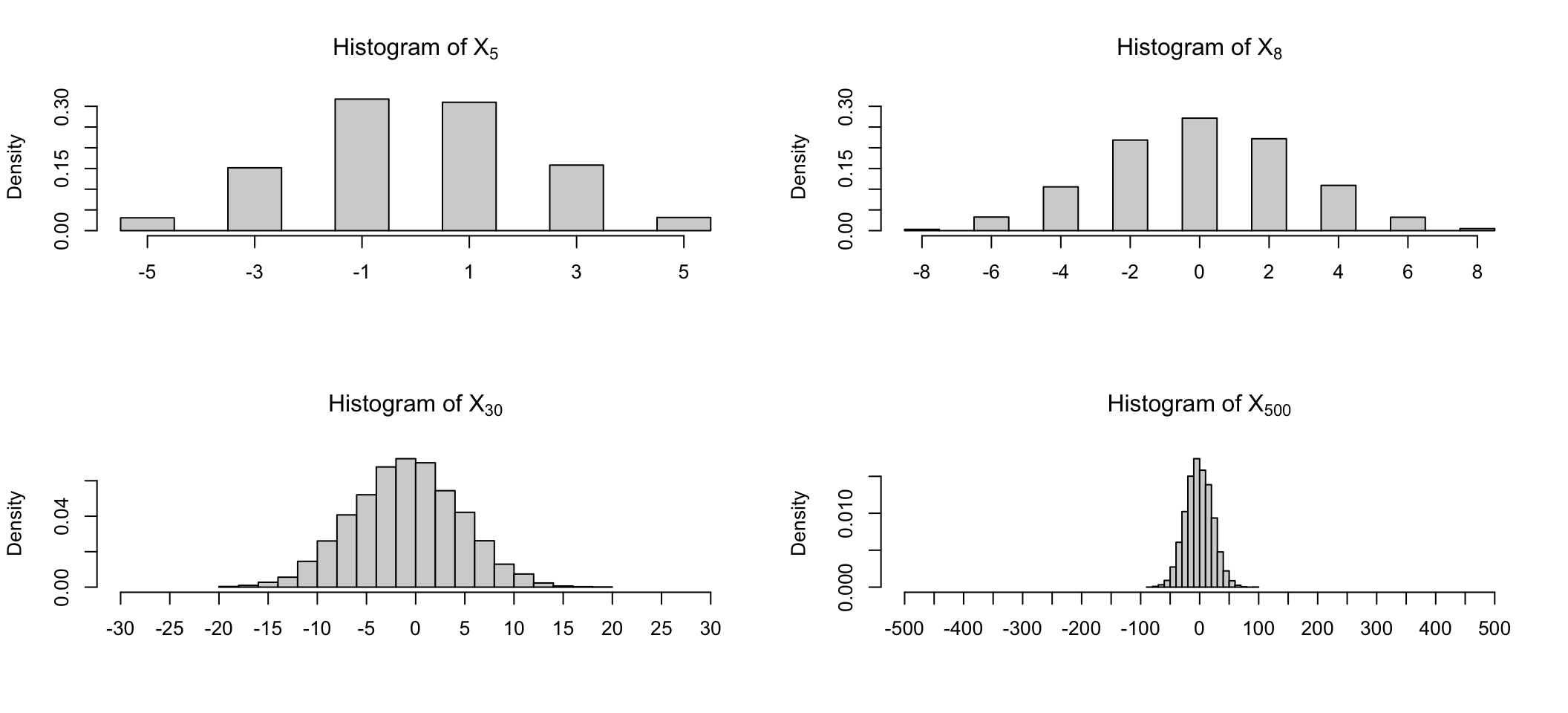
Here we focus on individual random variables (column) or pairs, triplets, etc. of random variables and study their (joint) distributions. For example, we can plot histograms of the random variables \(X_5, X_8, X_{30}\) or \(X_{500}\):

We can also use various (graphical or not) devices to understand joint distributions of pairs of random variables:

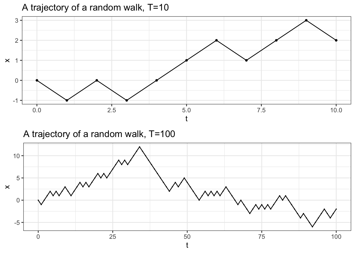
3.4.2 Row-wise (trajectorially or path-wise)

If we focus on what is going on in a given row of walk, we are going to see a different cross-section of our stochastic process. This way we are fixing the state of the world \(\omega\) (represented by a row of walk), i.e., the particular realization of our process, by varying the time parameter. A typical picture associated to a trajectory of a random walk is the following

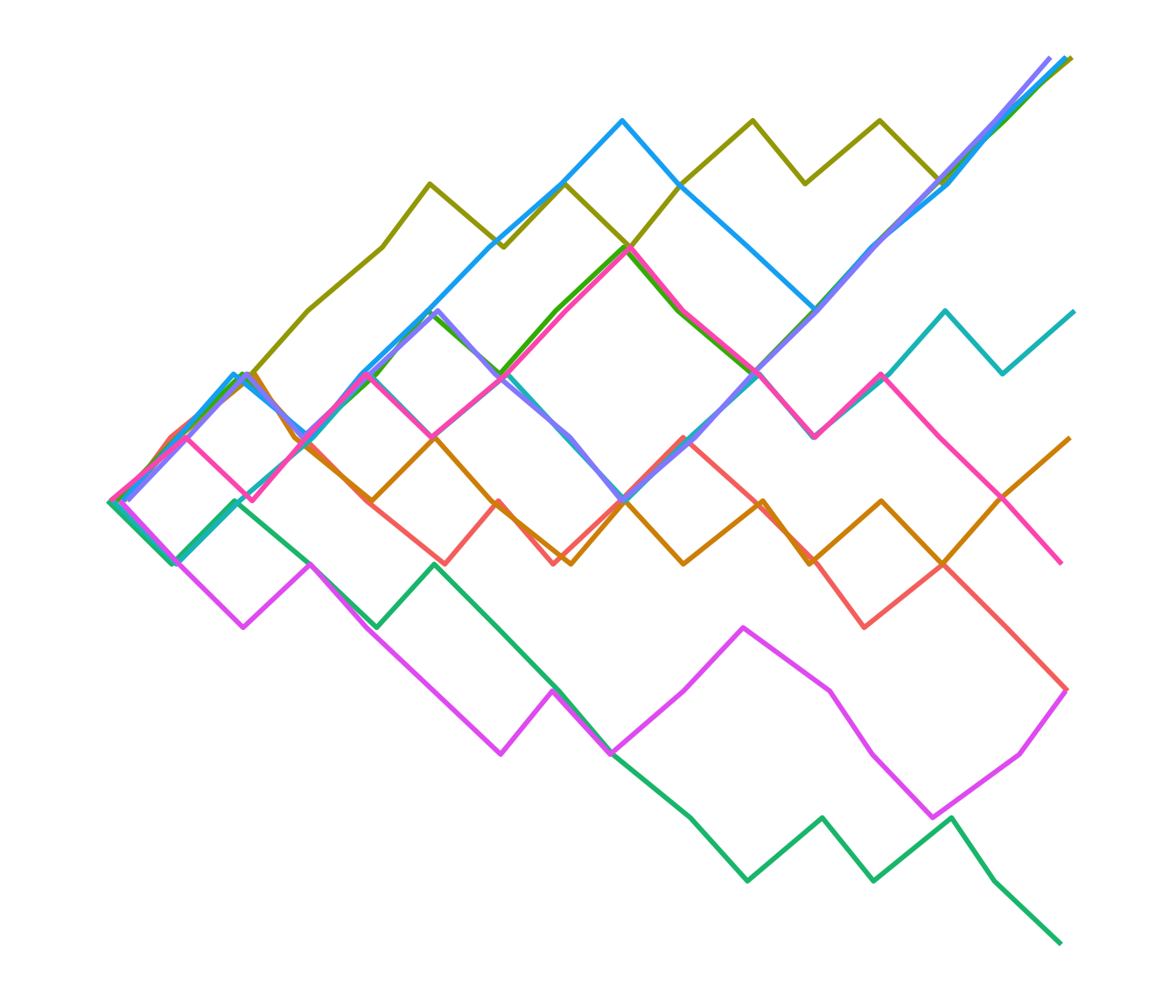
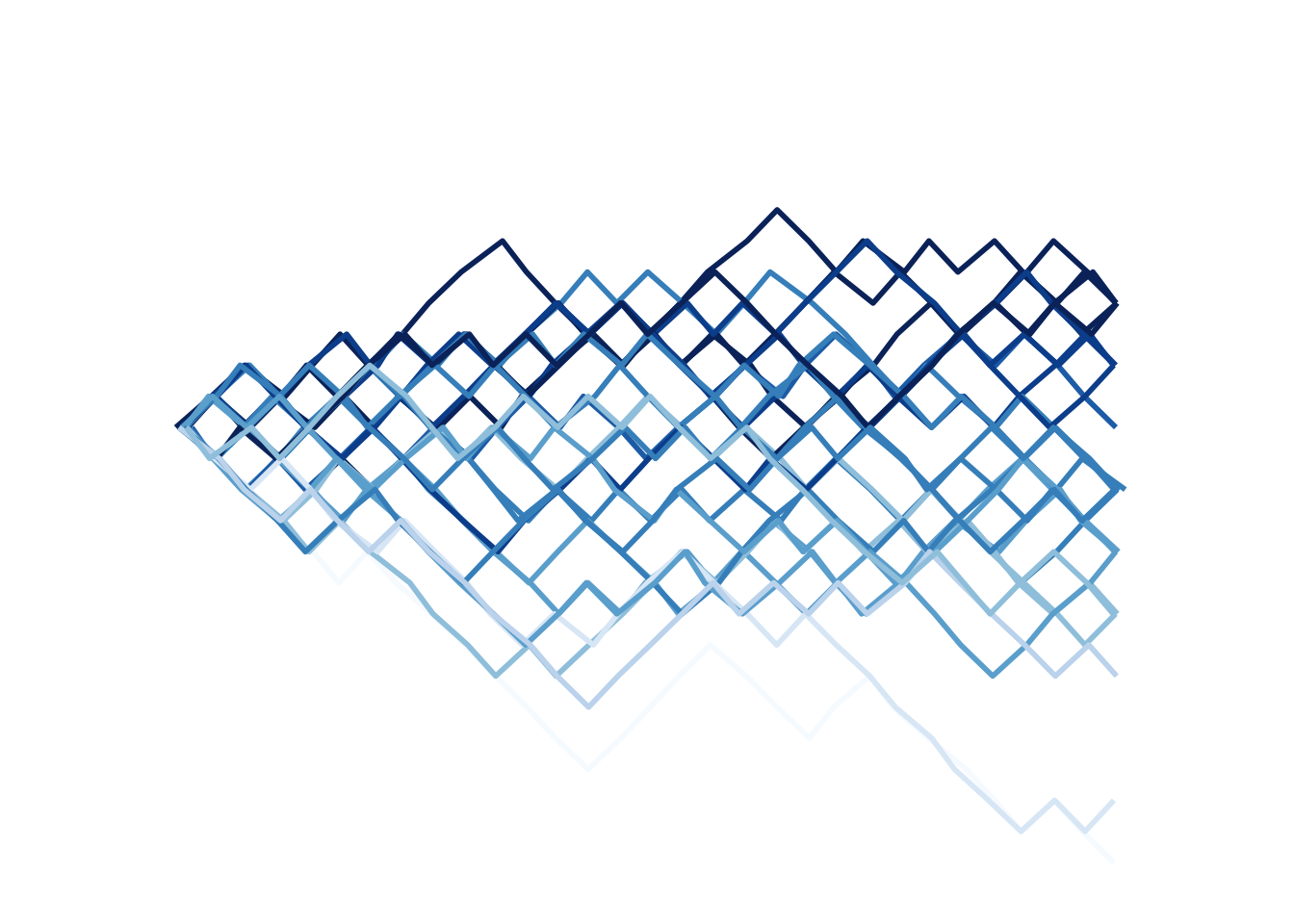
You can try to combine the two approaches (if you must) and plot several trajectories on the same plot. While this produces pretty pictures (and has one or two genuine applications), it usually leads to a sensory overload. Note that the trajectories on the righr are jittered a bit. That means that the positions of the points are randomly shifted by a small amount. This allows us to see features of the plot that would otherwise be hidden because of the overlap.

3.5 The path space

The row-wise (or path-wise or trajectory-wise) view of the random walk described above illustrates a very important point: the random walk (and random processes in general) can be seen as random “variable” whose values are not merely numbers; they are sequences of numbers (trajectories). In other words, a random process is simply a “random trajectory”. We can simulate this random trajectory as we did above, but simulating the steps and adding them up, but we could also take a different approach. We could build the set of all possible trajectories, and then pick a random trajectory out of it.

For a random walk on a finite horizon \(T\), a trajectory is simply a sequence of natural numbers starting from \(0\). Different realizations of the coin-tosses \(\delta_n\) will lead to different trajectories, but not every sequence of natural numbers corresponds to a trajectory. For example \((0,3,4,5)\) is not possible because the increments of the random walk can only take values \(1\) or \(-1\). In fact, a finite sequence \((x_0, x_1, \dots, x_T)\) is a (possible) sample path of a random walk if and only if \(x_0=0\) and \(x_{k}-x_{k-1} \in \{-1,1\}\) for each \(k\). For example, when \(T=3\), there are \(8\) possible trajectories: \[ \begin{align} \Omega = \{ &(0,1,2,3), (0,1,2,1),(0,1,0,2), (0,1,0,-1), \\ & (0,-1,-2,-3), (0,-1,-2,-1), (0,-1,0,-2), (0,-1,0,1)\} \end{align}\] When you (mentally) picture them, think of their graphs:

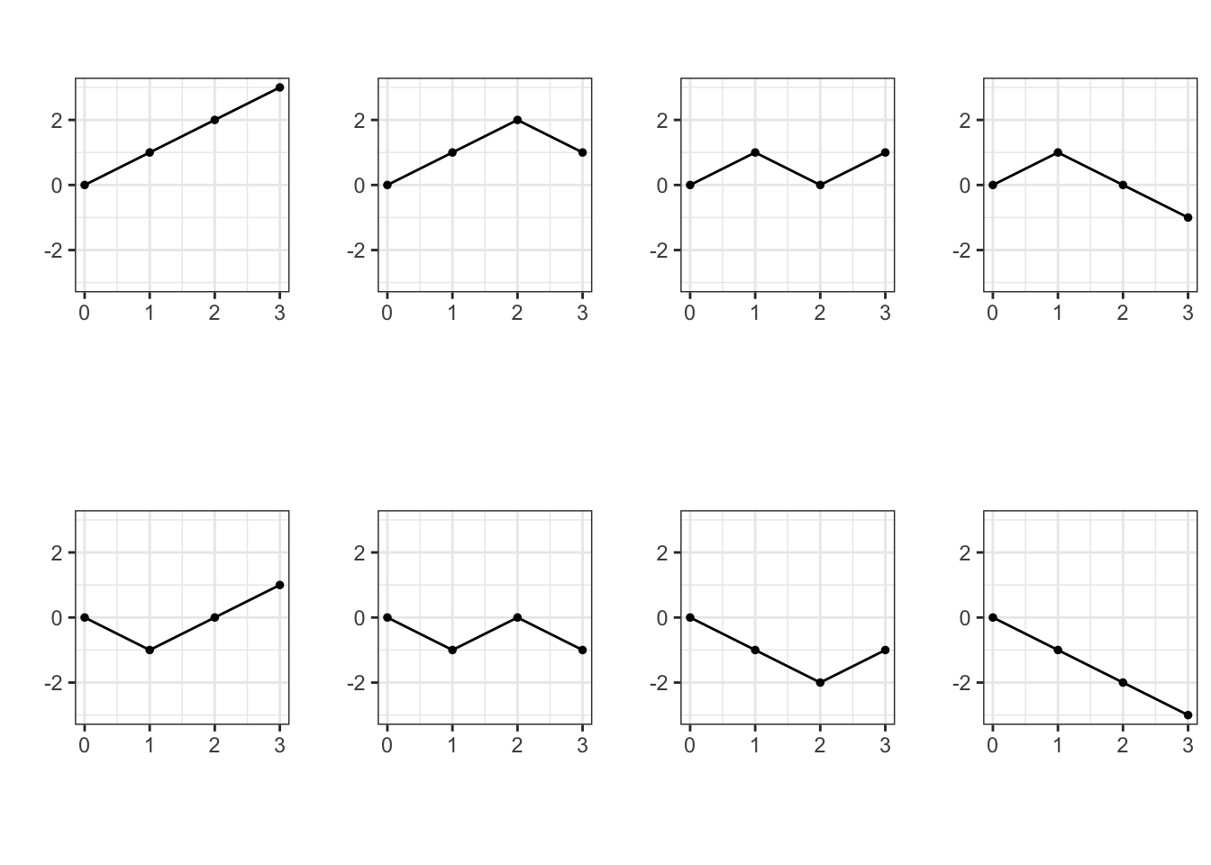
Each trajectory corresponds to a particular combination of the values of the increments \((\delta_1,\dots, \delta_T)\), each such combination happens with probability \(2^{-T}\). This means that any two trajectories are equally likely. That is convenient, because this puts uniform probability on the collection of trajectories. We are now ready to implement our simulation procedure in R; let us write the function single_trajectory using this approach and use it to simulate a few trajectories. We assume that a function all_paths(T) which returns a list of all possible paths with horizon \(T\) has already been implemented (more info about a possible implementation in R is given in a problem below):

T=5
Omega = all_paths(T)
single_trajectory = function() {
  return(unlist(sample(size=1,Omega)))
}

simulate_walk = function(nsim, p=0.5) {
   return(data.frame(
            X0=0, 
            t(replicate(nsim, single_trajectory()))
        ))
}

3.6 The distribution of \(X_n\)

Building a path space is not simply an exercise in abstraction. Here is how we can use is to understand the distribution of the position of the random walk:

Problem 3.1 Let \(X\) be a simple symmetric random walk with time horizon \(T=5\). What is the probability that \(X_{5}=1\)?

Solution. Let \(\Omega\) be the path space, i.e., the set of all possible trajectories of length \(5\) - there are \(2^{5}=32\) of them. The probability that \(X_{5}=1\) is the probability that a randomly picked path from \(\Omega\) will take the value \(1\) at \(n=5\). Since all paths are equally likely, we need to count the number of paths with value \(1\) at \(n=5\) and then divide by the total number of paths, i.e., \(32\).

So, how many paths are there that take value \(1\) at \(n=5\)? Each path is built out of steps of absolute value \(1\). Some of them go up (call them up-steps) and some of them go down (down-steps). A moment’s though reveals that the only way to reach \(1\) in \(5\) steps is if you have exactly \(3\) up-steps and \(2\) down-steps. Conversely, any path that has \(3\) up-steps and \(2\) down-steps ends at \(1\).

This realization transforms the problem into the following: how many paths are there with exactly \(3\) up-steps (note that we don’t have to specify that there are \(2\) down-steps - it will happen automatically). The only difference between different paths with exactly \(3\) up-steps is the position of these up-steps. In some of them the up-steps happen right at the start, in some at the very end, and in some they are scattered around. Each path with \(3\) up-steps is uniquely determined by the list of positions of those up-steps, i.e., with a size-\(3\) subset of \(\{1,2,3,4,5\}\). This is not a surprise at all, since each path is built out of increments, and positions of positive increments clearly determine values of all increments.

The problem has now become purely mathematical: how many size-\(3\) subsets of \(\{1,2,3,4,5\}\) are there? The answer comes in the form of a binomial coefficient \(\binom{5}{3}\) whose value is \(10\) - there are exactly ten ways to pick three positions out of five. Therefore, \[ {\mathbb{P}}[ X_{5} = 1] = 10 \times 2^{-5} = \frac{5}{16}.\]

Can we do this in general?

Problem 3.2 Let \(X\) be a simple symmetric random walk with time horizon \(T\). What is the probability that \(X_{n}=k\)?

Solution. The reasoning from the last example still applies. A trajectory with \(u\) up-steps and \(d\) down-steps will end at \(u-d\), so we must have \(u-d=k\). On the other hand \(u+d=n\) since all steps that are not up-steps are necessarily down-steps. This gives as a simple linear system with two equations and two unknowns which solves to \(u = (n+k)/2\), \(d=(n-k)/2\). Note the \(n\) and \(k\) must have the same parity for this solution to be meaningful. Also, \(k\) must be between \(-n\) and \(n\).

Having figured out how many up-steps is necessary to reach \(k\), all we need to do is count the number of trajectories with that many up-steps. Like before, we can do that by counting the number of ways we can choose their position among \(n\) steps, and, like before, the answer is the binomial coefficient \(\binom{n}{u}\) where \(u=(n+k)/2\). Dividing by the total number of trajectories gives us the final answer: \[ {\mathbb{P}}[ X_n = k ] = \binom{n}{ (n+k)/2} 2^{-n},\] for all \(k\) between \(-n\) and \(n\) with same parity as \(n\). For all other \(k\), the probability is \(0\).

The binomial coefficient and the \(n\)-th power suggest that the distribution of \(X_n\) might have something to do with the binomial distribution. It is clearly not the binomial, since it can take negative values, but it is related. To figure out what is going on, let us first remember what the binomial distribution is all about. Formally, it is a discrete distribution with two parameters \(n\in{\mathbb{N}}\) and \(p\in (0,1)\). Its support is \(\{0,1,2,\dots, n\}\) and the distribution is given by the following table, where \(q=1-p\)

0	1	2	…	k	…	n
\(\binom{n}{0} q^n\)	\(\binom{n}{1} p q^{n-1}\)	\(\binom{n}{2} p^2 q^{n-2}\)	…	\(\binom{n}{k} p^k q^{n-k}\)	…	\(\binom{n}{n} p^n\)

The binomial distribution is best understood, however, when it is expressed as a “number of successes”. More precisely,

If \(B_1,B_2,\dots, B_n\) are \(n\) independent Bernoulli random variables with the same parameter \(p\), then their sum \(B_1+\dots+B_n\) has a binomial distribution with parameters \(n\) and \(p\).

We think of \(B_1, \dots, B_n\) as indicator random variables of “successes” in \(n\) independent “experiments” each of which “succeeds” with probability \(p\). A canonical example is tossing a biased coin \(n\) times and counting the number of “heads”.

We know that the position \(X_n\) at time \(n\) of the random walk admits the representation \[ X_n = \delta_1+\delta_2+\dots+\delta_n,\] just like the binomial random variable. The distribution of \(\delta_k\) is not Bernoulli, though, since it takes the values \(-1\) and \(1\), and not \(0,1\). This is easily fixed by applying the linear transformation \(x\mapsto \frac{1}{2}(x+1)\); indeed \(( -1 +1)/2 = 0\) and \(( 1 + 1) / 2 =1\), and, so, \[ \frac{1}{2}(\delta_k+1)\text{ is a Bernoulli random variable with parameter } p=\frac{1}{2}.\] Consequently, if we add all \(B_k = \tfrac{1}{2}(1+\delta_k)\) and remember our discussion from above we get the following statement

In a simple symmetric random walk the random variable \(\frac{1}{2} (n + X_n)\) has the binomial distribution with parameters \(n\) and \(p=1/2\), for each \(n\).

Can you use that fact to rederive the distribution of \(X_n\)?

3.7 Biased random walks

If the steps of the random walk preferred one direction to the other, the definition would need to be tweaked a little bit and the word “symmetric” in the name gets replaced by “biased” (or “asymmetric”):

A stochastic process \(\{X\}_{n\in{\mathbb{N}}_0}\) is said to be a **simple biased random walk with parameter \(p\in (0,1)\) if

\(X_0=0\),
the random variables \(\delta_1 = X_1-X_0\), \(\delta_2 = X_2 - X_1\), …, called the steps of the random walk, are independent and
each \(\delta_n\) has a biased coin-toss distribution, i.e., its distribution is given by \[{\mathbb{P}}[ \delta_n = 1] = p \text{ and } {\mathbb{P}}[ \delta_n=-1] = 1-p \text{ for each } n.\]

As far as the distribution of \(X_n\) is concerned, we don’t expect it to be the same as in the symmetric case. After all, the biased random walk (think \(p=0.999\)) will prefer one direction over the other. Our trick with writing \(\frac{1}{2}(n+X_n)\) as a sum of Bernoulli random variables still works. We just have to remember that \(p\) is not \(\frac{1}{2}\) anymore to conclude that \(\tfrac{1}{2}(X_n + n)\) has the binomial distribution with parameters \(n\) and \(p\); if we put \(u = (n+k)/2\) we get \[\begin{align} {\mathbb{P}}[ X_n = k] &= {\mathbb{P}}[ \tfrac{1}{2}(X_n+n) = u] = \binom{n}{u} p^u q^{n-u}\\ & = \binom{n}{\frac{1}{2}(n+k)} p^{\frac{1}{2}(n+k)} q^{\frac{1}{2}(n-k)}. \end{align}\] Note that be binomial coefficient stays the same as in the symmetric case, but the factor \(2^{-n} = (1/2)^{\frac{1}{2}(n+k)} (1/2)^{\frac{1}{2}(n-k)}\) becomes \(p^{\frac{1}{2}(n+k)} q^{\frac{1}{2}(n-k)}\).

Can we reuse the sample space \(\Omega\) to build a biased random walk? Yes, we can, but we need to assign possibly different probabilities to individuals. Indeed, if \(p=0.99\), the probability that all the increments \(\delta\) of a \(10\)-step random walk take the value \(+1\) is \((0.99)^{10} \approx 0.90\). This is much larger than the probability that all steps take the value \(-1\), which is \((0.01)^{10}= 10^{-20}\).

In general, the probability that a particular path is picked out of \(\Omega\) will depend on the number of up-steps and down-steps; more precisely it equals \(p^u q^{n-u}\) where \(u\) is the number of up-steps. The interesting thing is that the number of up-steps \(u\) depends only on the final position \(x_n\) of the path; indeed \(u = \frac{1}{2}(n+x_n)\). This way, all paths of length \(T=5\) that end up at \(1\) get the same probability of being chosen, namely \(p^3 q^2\). Let us use the awful seizure-inducing graph with multiple paths for good, and adjust the each path according to its probability; some jitter has been added to deal with overlap. The lighter-colored paths are less likely to happen then the darker-colored paths.

3.8 Additional problems for Chapter 3

Problem 3.3 Let \(\{X_n\}_{n\in {\mathbb{N}}_0}\) be a simple symmetric random walk. Which of the following processes are simple random walks?

\(\{2 X_n\}_{n\in {\mathbb{N}}_0}\) ?
\(\{X^2_n\}_{n\in {\mathbb{N}}_0}\) ?
\(\{-X_n\}_{n\in {\mathbb{N}}_0}\) ?
\(\{ Y_n\}_{n\in {\mathbb{N}}_0}\), where \(Y_n = X_{5+n}-X_5\) ?

How about the case \(p\ne \tfrac{1}{2}\)?

Click for Solution

Solution.

No - the support of the distribution of \(X_1\) is \(\{-2,2\}\) and not \(\{-1,1\}\).
No - \(X_1^2=1\), and not \(\pm 1\) with equal probabilities.
Yes - all parts of the definition check out.
Yes - all parts of the definition check out.

The answers are the same if \(p\ne \tfrac{1}{2}\), but, in 3., \(-X_n\) comes with probability \(1-p\) of an up-step, and not \(p\).

Problem 3.4 Let \(\{X_n\}_{n\in {\mathbb{N}}_0}\) be a simple random walk.

Find the distribution of the product \(X_1 X_2\)
Compute \({\mathbb{P}}[ |X_1 X_2 X_3|]=2\)
Find the probability that \(X\) will hit neither the level \(2\) nor the level \(-2\) until (and including) time \(T=3\)
Find the independent pairs of random variables among the following choices:
- \(X_1\) and \(X_2\)
- \(X_4 - X_2\) and \(X_3\)
- \(X_4 - X_2\) and \(X_6 - X_5\)
- \(X_1+X_3\) and \(X_2+X_4\).

Click for Solution

Solution.

The possible paths when the time horizon is \(T=2\) are \[(0,1,2), (0,1,0), (0,-1,-2) \text{ and } (0,-1,0)\] The values of the product \(X_1 X_2\) on those paths are \(2, 0, 2\), and \(0\), respectively. Each happens with probability \(0.25\). Therefore \({\mathbb{P}}[ X_1 X_2 = 0] = {\mathbb{P}}[ X_1 X_2 = 2] = \tfrac{1}{2}\), i.e., its distribution is given by

0	2
0.5	0.5

\(|X_1 X_2 X_3|=2\) only in the following two cases \[ X_1=1, X_2=2, X_3=1 \text{ or } X_1=-1, X_2=-2, X_3=-1.\] Each of those paths has probability \(1/8\) of happening, so \({\mathbb{P}}[ |X_1 X_2 X_3| = 2] = 1/4\).
The only chance for \(X\) to hit \(2\) or \(−2\) before or at T = 3 is at time \(n = 2\). Since \(X_2 \in \{ -2, 0, 2\}\), this happens with probability \({\mathbb{P}}[ X_2 \in \{-2,2\}] = 1 - {\mathbb{P}}[X_2 = 0] = 0.5\).
The only independent pair is \(X_4 - X_2\) and \(X_6 - X_5\) because the two random variables are build out of completely different increments: \(X_4 - X_2 = \delta_3+\delta_4\) while \(X_6-X_5 = \delta_6\). The others are not independent. For example, if we are told that \(X_1+X_3 = 4\), it necessarily follows that \(\delta_1= \delta_2=\delta_3=1\). Hence, \(X_2+X_4 = 2\delta_1+2\delta_2+\delta_3+\delta_4 = 5+\delta_4\) which cannot be less than \(4\). On the other hand, without any information, \(X_2+X_4\) can easily be negative.

Problem 3.5 Let \(\{X_n\}_{n\in {\mathbb{N}}_0}\) be a simple random walk.

Compute \({\mathbb{P}}[ X_{32} = 4| X_8 = 6]\).
Compute \({\mathbb{P}}[ X_9 = 3 \text{ and } X_{15}=5 ]\)
(extra credit) Compute \({\mathbb{P}}[ X_7 + X_{12} = X_1 + X_{16}]\)

Click for Solution

Solution.

This is the same as \({\mathbb{P}}[ X_{32}- X_8 = -2 | X_8=6]\). The random variables \(X_8\) and \(X_{32}-X_8\) are independent (as they are built out of different \(\delta\)s), so we can remove the conditioning. It remains to compute \({\mathbb{P}}[X_{32} - X_8 = -2]\). For that, we note that \(X_{32} - X_8\) is a sum of \(24\) independent coin tosses, so its distribution is the same as that of \(X_{24}\). Therefore, by our formula for the distribution of \(X_n\), we have \[ {\mathbb{P}}[X_{32}= 4 | X_8 = 6] = {\mathbb{P}}[X_{24} = -2] = \binom{24}{11} 2^{-24}.\]
We have \[\begin{align} {\mathbb{P}}[ X_9 = 3 \text{ and } X_{15}=5 ] & = {\mathbb{P}}[ X_{15} = 5 | X_9 = 3] \times {\mathbb{P}}[ X_9=3] \\ & = {\mathbb{P}}[ X_6 = 2] \times {\mathbb{P}}[X_9=3] = \binom{6}{4} 2^{-6} \binom{9}{6} 2^{-9}, \end{align}\] where we used the same ideas as in 1. above
We rewrite everything using \(\delta\)s: \[\begin{align} X_7+X_{12} = X_1+X_{16} &\Leftrightarrow X_7-X_1 = X_{16}-X_{12} \Leftrightarrow \delta_2+\dots+\delta_7 = \delta_{13} + \dots+\delta_{16}\\ & \Leftrightarrow (-\delta_2) + \dots + (-\delta_7) + \delta_{13}+ \dots + \delta_{16} = 0. \end{align}\] Since \(-\delta_k\) has the same distribution as \(\delta_k\) (both are coin tosses) and remains independent of all other \(\delta_i\), the left-hand side of the last expression in the chain of equivalences above is a sum of \(10\) indepenedent coin tosses. Therefore, the probability that it equals \(0\) is the same as \({\mathbb{P}}[X_{10}=0] = \binom{10}{5} 2^{-10}\).

Problem 3.6 Let \(\{X_n\}_{n\in {\mathbb{N}}_0}\) be a simple random walk. For \(n\in{\mathbb{N}}\) compute the probability that \(X_{2n}\), \(X_{4n}\) and \(X_{6n}\) take the same value.

Click for Solution

Solution. Increments \(X_{4n}-X_{2n}\) and \(X_{6n} - X_{4n}\) are independent, and each is a sum of \(2n\) independent coin tosses (therefore has the same distribution as \(X_{2n}\)). Hence, \[\begin{aligned} {\mathbb{P}}[ X_{2n} = X_{4n} \text{ and }X_{4n} = X_{6n} ] &= {\mathbb{P}}[ X_{4n} - X_{2n} = 0 \text{ and }X_{6n} - X_{4n} = 0 ]\\ &= {\mathbb{P}}[ X_{4n} - X_{2n} = 0] \times {\mathbb{P}}[ X_{6n} - X_{4n}=0]\\ &={\mathbb{P}}[ X_{2n}=0] \times {\mathbb{P}}[ X_{2n} =0 ]\\ & = \binom{2n}{n} 2^{-2n} \binom{2n}{n} 2^{-2n} = \binom{2n}{n}^2 2^{-4n}. \end{aligned}\]

Problem 3.7 (Extra Credit) Write an R function (call it all_paths) which takes an integer argument T and returns a list of all possible paths of a random walk with time horizon \(T\). (Note: Since vectors cannot have other vectors as elements, you will need to use a data structure called list for this. It behaves very much like a vector, so it should not be a problem.)

Click for Solution

Solution. The implementation below uses the function combn which returns the list of all subsets of a certain size of a certain vector. Since each path is determined by the positions of its up-steps, we need to loop through all numbers \(i\) from \(0\) to \(T\) and then list all subsets of the size \(i\). The next step is to turn a set of positions to a path of a random walk. This can be done in many ways; one is implemented implemented in choice_to_path using vector indexing.

choice_to_path = function(comb, T) {
    increments = rep(-1, T)
    increments[comb] = 1
    path = cumsum(increments)
    return(path)
}

all_paths = function(T) {
    Omega = list(2^T)
    index = 1
    for (i in 0:T) {
        choices = combn(T, i, simplify = FALSE)
        for (choice in choices) {
            Omega[[index]] = choice_to_path(choice, T)
            index = index + 1
        }
    }
    return(Omega)
}

Problem 3.8 Let \(\{X_n\}_{n\in {\mathbb{N}}_0}\) be a simple symmetric random walk. Given \(n\in{\mathbb{N}}_0\) and \(k\in{\mathbb{N}}\), compute \(\operatorname{Var}[X_n]\), \(\operatorname{Cov}[X_n, X_{n+k}]\) and \(\operatorname{corr}[X_n, X_{n+k}]\), where \(\operatorname{Cov}\) stands for the covariance and \(\operatorname{corr}\) for the correlation. (Note: look up \(\operatorname{Cov}\) and \(\operatorname{corr}\) if you forgot what they are).

Compute \(\lim_{n\to\infty} \operatorname{corr}[X_n, X_{n+k}]\) and \(\lim_{k\to\infty} \operatorname{corr}[X_n, X_{n+k}]\). How would you interpret the results you obtained?

Click for Solution

Solution. We have \(\operatorname{Var}[\delta_i] = 1\) for each \(i\in{\mathbb{N}}\), so \[\operatorname{Var}[X_n] = \sum_{i=1}^n \operatorname{Var}[\delta_i] = n.\] Since \({\mathbb{E}}[X_n] = {\mathbb{E}}[X_{n+k}]=0\) and \(X_{n+k} - X_n\) is independent of \(X_n\), we have \[\begin{aligned} \operatorname{Cov}[X_n,X_{n+k}] &= {\mathbb{E}}[ X_n X_{n+k}] = {\mathbb{E}}[ X_n (X_{n+k} - X_n)] + {\mathbb{E}}[X_n^2] = {\mathbb{E}}[X_n] {\mathbb{E}}[X_{n+k} - X_n] + {\mathbb{E}}[X_n^2]\\ &= {\mathbb{E}}[X_n^2] = n. \end{aligned}\] Finally, \[\begin{aligned} \operatorname{corr}[X_n, X_{n+k}] = \frac{\operatorname{Cov}[X_n, X_{n+k}]}{\sqrt{\operatorname{Var}[X_n]} \sqrt{\operatorname{Var}[X_{n+k}]}} = \frac{n}{\sqrt{n(n+k)}} = \sqrt{\frac{n}{n+k}}. \end{aligned}\] When we let \(n\to\infty\), we get \(1\). This means that the positions of the random walk, \(k\) steps apart, get closer and close to perfect correlation as \(n\to\infty\). If you know \(X_n\) and \(n\) is large, you almost know \(X_{n+k}\), at least at the typical scale of \(X_n\).

When we let \(k\to\infty\), we get \(0\). That means that as the gap between two points in time gets larger, the values get less and less correlated. In a sense, the random walk tends to forget its past after a large number of steps.

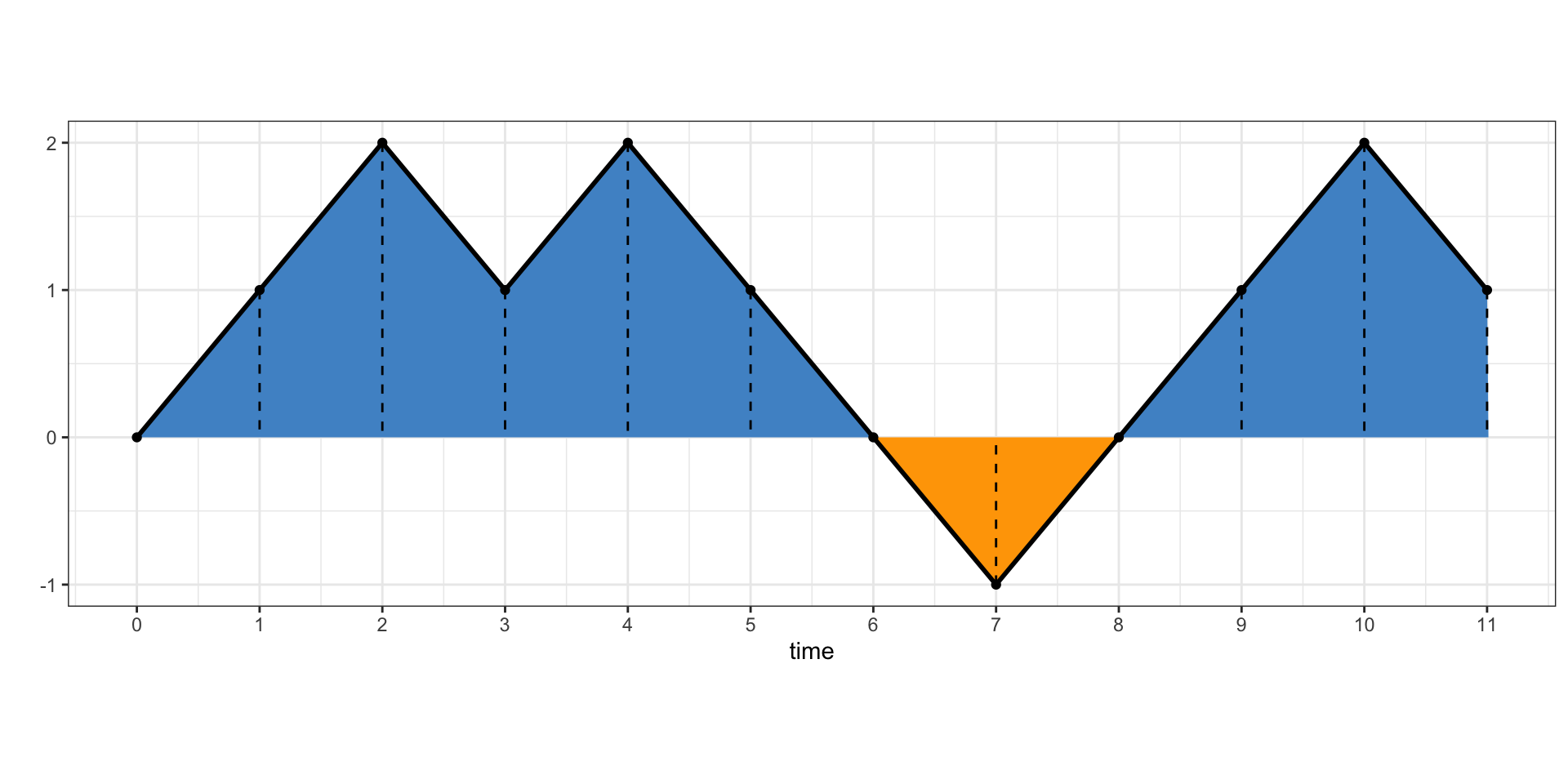
Problem 3.9 Let \(\{X_n\}_{n\in {\mathbb{N}}_0}\) be a simple random walk with \({\mathbb{P}}[X_1=1]=p\in (0,1)\), and let \(A_n\) be the (signed) area under its graph (in the picture below, \(A_n\) is the area of the blue part minus the area of the orange part).

Find a formula for \(A_n\) in terms of \(X_1,\dots, X_n\).
Compute \({\mathbb{E}}[A_n]\) and \(\operatorname{Var}[A_n]\), for \(n\in{\mathbb{N}}\). (You will find the following formulas helpful \(\sum_{j=1}^n j = \frac{n(n+1)}{2}\) and \(\sum_{j=1}^n j^2=\frac{n(n+1)(2n+1)}{6}\).)
Use simulations to approximate the entire distribution of \(A_n\) (set \(p=0.3\), \(n=10\) run \(10000\) simulations): display the entire distribution table. Next, compute Monte-Carlo approximations to \({\mathbb{E}}[A_{10}]\) and \(\operatorname{Var}[A_{10}]\) and compare them to the exact values obtained in 2. above.

Click for Solution

Solution.

The dashed lines divide the area “under” the graph in separate trapezoids, so \(A_n\) is the sum of their areas. The trapezoid between \(X_{k-1}\) and \(X_{k}\) has area \(1 \times (X_{k-1}+X_{k})/2\), so \[ A_n = \sum_{k=1}^n \tfrac{1}{2} (X_{k-1}+X_k) = X_1+X_2+\dots+X_{n-1} + \tfrac{1}{2}X_n.\]
Let us first represent \(A_n\) in terms of the sequence \(\{\delta_n\}_{n\in{\mathbb{N}}_0}\) \[\begin{align} A_n &= (\delta_1) + (\delta_1+\delta_2) + \dots + (\delta_1+\dots + \delta_{n-1}) + \tfrac{1}{2}(\delta_1+ \dots + \delta_n)\\ &= (n-\tfrac{1}{2}) \delta_1 + (n-1-\tfrac{1}{2}) \delta_2 + \dots + \tfrac{1}{2}\delta_n. \end{align}\] We compute \({\mathbb{E}}[\delta_k]=p-q\) so that, by the formulas from the problem, \[\begin{align} {\mathbb{E}}[A_n]&= \sum_{j=1}^n (j-\tfrac{1}{2}) {\mathbb{E}}[\delta_{n-j}] = (p-q) \Big( \tfrac{1}{2}n(n+1) - \tfrac{1}{2}n\Big)\\ & = \frac{p-q}{2} n^2 \end{align}\] Just like above, but relying on the independence of \(\{\delta_n\}\) and the fact that \(\operatorname{Var}[\delta_k]=1-(2p-1)^2=4pq\), we have \[\begin{align} \operatorname{Var}[A_n] &= \sum_{j=1}^n \operatorname{Var}[(j - \tfrac{1}{2}) \delta_{n-j}] = \sum_{j=1}^n (j-\tfrac{1}{2})^2 \operatorname{Var}[\delta_k] \\& = 4pq \sum_{j=1}^n (j-\tfrac{1}{2})^2 = 4pq \Big( \sum_{j=1}^n j^2 - \sum_{j=1}^n j + \frac{1}{4} n \Big)\\ & = 4pq \Big( \frac{n}{n+1}{(2n+1)}{6} - \frac{n (n+1)}{2} + \frac{n}{4}) = \frac{pq}{3} ( 4 n^3 - n) \end{align}\]

First, we draw \(10000\) simulations of a simple random walk. For that we use the function simulate_walk from the notes above:

walk = simulate_walk(nsim = 10000, T = 6, p = 0.3)

Next, we use the formula \(A_{6} = X_1+ \dots+X_5 + \tfrac{1}{2}X_{6}\) from 1. to create the vector A6, which will hold \(10000\) simulations of \(A_{6}\). We use the function apply to apply the function sum to each row of walk (that is what the MARGIN = 1 argument means; settingMARGIN = 2, would produce the vector of column sums):

A6 = apply(walk, MARGIN = 1, FUN = sum) - 0.5 * walk$X6

Next, we create the table of relative frequencies of occurrences of each value in A6. This table will serve as an approximation to the true distribution of \(A_{6}\):

(dist_est = prop.table(table(A6)))
## A6
##    -18    -17    -15    -14    -13    -12    -11    -10     -9     -8     -7 
## 0.1223 0.0503 0.0510 0.0199 0.0529 0.0233 0.0515 0.0415 0.0608 0.0429 0.0540 
##     -6     -5     -4     -3     -2     -1      0      1      2      3      4 
## 0.0675 0.0169 0.0407 0.0293 0.0468 0.0269 0.0275 0.0278 0.0317 0.0278 0.0076 
##      5      6      7      8      9     10     11     12     13     14     15 
## 0.0169 0.0103 0.0112 0.0073 0.0112 0.0087 0.0015 0.0036 0.0019 0.0034 0.0012 
##     17     18 
## 0.0014 0.0005

Using the formulas derived in 2. above, we get the following exact values \[\begin{align} {\mathbb{E}}[A_6]&= \frac{0.3 - 0.7}{2} 6^2 = - 7.5 \\ \operatorname{Var}[A_6] & \frac{0.3 \times 0.7}{3} ( 4 6^3 - 6) = 60.06, \end{align}\]

and Monte Carlo gives us the following estimates and their relative errors:

(expectation_true = -7.5)
## [1] -7.5
(expectation_est = mean(A6))
## [1] -7.3
(variance_true = 60.06)
## [1] 60
(variance_est = sd(A6)^2)
## [1] 60
(rel_error_expectation = (expectation_true - expectation_est)/expectation_true)
## [1] 0.024
(rel_error_variance = (variance_true - variance_est)/variance_true)
## [1] 0.0079

Problem 3.10 Let \(\{X_n\}_{0 \leq n \leq 100}\) be the simple symmetric random walk with time horizon \(T = 100\). We define the following random variables

\(L\) is the time of the last zero, i.e., the last time, before or at \(T\), that \(X\) visited \(0\)
\(P\) is the amount of time spent above \(0\) i.e., the number of all times \(n\leq T\) with \(X_n>0\).
\(R\) is the last time time the maximum is attained, i.e., the last time before or at \(T\), that \(X\) took the value \(M_T\), where \(M\) is the running maximum process associated to \(X\).

Draw nsim simulations of \(L\), \(P\) and \(R\) and display their histograms on the same graph, side by side. Set the number of bins (option breaks in the command hist) to \(50\). Choose the number nsim so that the simulations take no more than 2 minutes, but do not go over \(100,000\).

(Hint: For each of the three random variables write a function which takes a single trajectory of a random walk as an argument and returns its value for that trajectory. \(P\) is easy, and for \(L\) and \(R\) use the function match. Be careful - match finds the first match, but you need the last one. Then simulate the random walk and apply your functions to the rows of your ouput data frame.)
What do you observe? What conjecture can you make about distributions of \(L\), \(P\) and \(R\)?
(Extra credit) Even though \(L\), \(P\) and \(R\) are discrete random variables, it turns out that distributions of their normalized versions \(L/T\), \(P/T\) and \(R/T\) are close to named continuous distributions. Guess what these distributions are and explain (graphically) why you think your guess is correct.

Click for Solution

Solution.

First, we simulate nsim=100,000 trajectories of length T=100 of a simple symmetric random walk. We reuse the function simulate_walk from the notes.

T = 100
nsim = 100000
df = simulate_walk(nsim, T)

Next, we write three functions. The input to each will be a trajectory of a random walk, and the output will be the value of the corresponding random variable (\(P\), \(L\) or \(R\)) for that particular trajectory. The function rev reverses its input.

compute_P = function(x) {
    p = sum(x > 0)
    return(p)
}

compute_L = function(x) {
    L = length(rev(x)) - match(0, rev(x)) + 1
    return(L)
}

compute_R = function(x) {
    R = length(rev(x)) - match(max(x), rev(x)) + 1
    return(R)
}

Then we apply each of the functions to each row of df (the data frame that holds simulated trajectories of the walk)

R = apply(df, 1, compute_R)
L = apply(df, 1, compute_L)
P = apply(df, 1, compute_P)

and plot the histograms (ylim sets the visible range of the \(y\) axis. We make all three the same in order be able to compare the histograms better)

par(mfrow = c(1, 3))
hist(R, breaks = 50, prob = T, ylim = c(0, 0.04))
hist(L, breaks = 50, prob = T, ylim = c(0, 0.04))
hist(P, breaks = 50, prob = T, ylim = c(0, 0.04))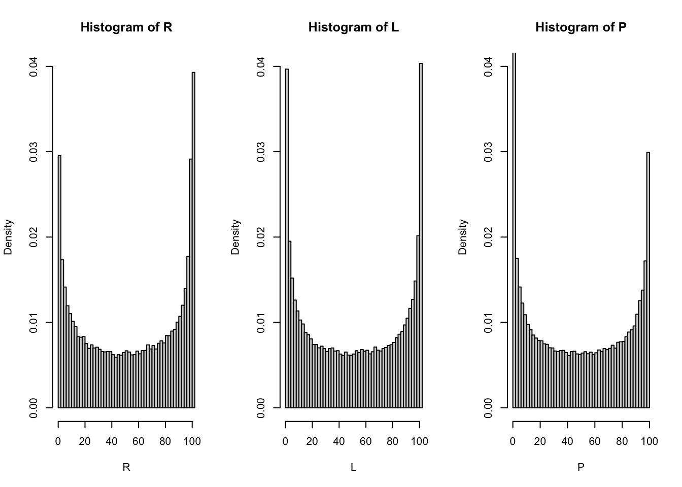

All three histograms look the same. Perhaps the random variables \(P\), \(L\) and \(R\) have the same distributions? That is quite strange, though, because they are constructed by very different procedures.
When we normalize the random variables \(P\),\(L\), and \(R\) by \(T=100\), i.e., consider \(P/100\), \(L/100\) and \(R/100\), we obtain almost the same histograms. The only difference is that the \(x\)-axis ranges from \(0\) to \(1\) and not from \(0\) to \(T=100\). This suggests to try and see if any of the named distributions with support on \([0,1]\) fits. Fortunately, there is only one non-esotheric family of distributions on \([0,1]\) and that is the beta family. If you fiddle around a bit with the two parameters you will quickly find that setting both of them to \(1/2\) fits our histograms very well (I am plotting only the histogram of \(R/T\); the others look very similar)
```
hist(R/100, breaks = 50, prob = T, main = "Histogram of R/100 with the pdf of B(1/2, 1/2) superimposed")
curve(dbeta(x, shape1 = 0.5, shape2 = 0.5), from = 0, to = 1, add = TRUE, col = 2,
    lwd = 2)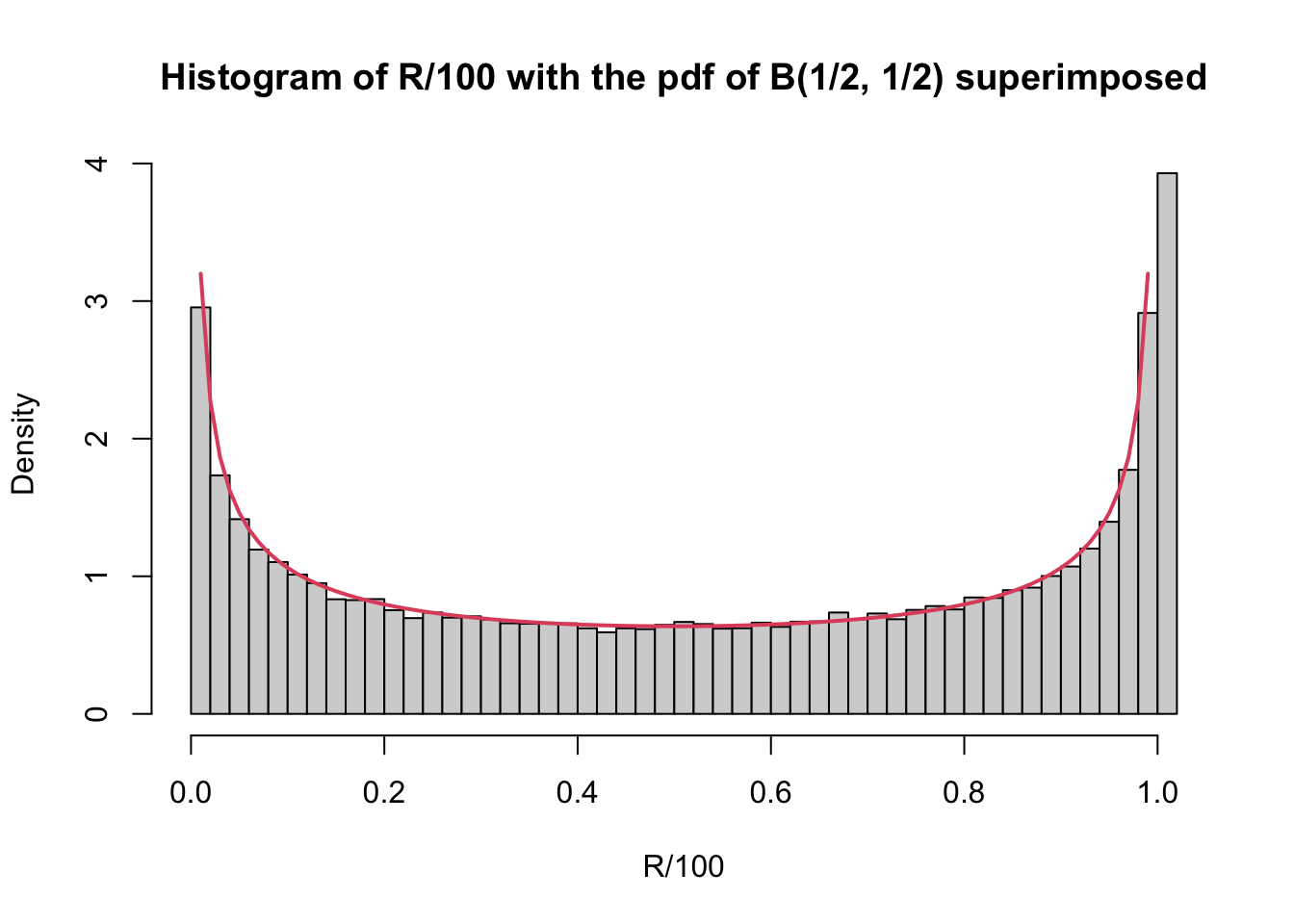
```
That is, indeed, what is going on. As the number of steps \(T\) gets larger, the distributions of \(L/,T\) \(P/T\) and \(R/T\) all converge towards the same, beta, distribution with parameters \(\alpha=1/2\) and \(\beta=1/2\). The exact meaning of the word “converge” in the previous sentence, or the proof of this statement are beyond the scope of this course, but you cannot argue with the fact that the fit looks really good on the picture above.

Btw, the pdf of the \(B(1/2,1/2)\) distribution is given by \[\begin{align} f(x) = \frac{1}{\pi \sqrt{x(1-x)}} \text{ for } x \in [0,1]. \end{align}\] The cdf \(F\) of \(B(1/2,1/2)\) is therefore given by \[\begin{align} F(x) = \int_0^x \frac{1}{\pi\sqrt{y(1-y)}}\, dy = \frac{2}{\pi} \arcsin(\sqrt{x}) \text{ for } x\in [0,1]. \end{align}\] This is why the \(B(1/2,1/2)\)-distribution is sometimes called the arcsine-distribution and the mathematical theorem that states that \(P/T\), \(L/T\) and \(R/T\) all approach the \(B(1/2,1/2)\)-distribution as \(T\to\infty\) is called the arcsine law.

If you are interested in sports modeling, have a look at the following article where the arcsine law appears in an unusual context.

3.9 Endnotes

It is somewhat unfortunate that the standard notation for the time horizon, namely \(T\), coincides with a shortcut T for TRUE in R. Our example still works fine because this shortcut is used only if there is no variable named T.↩︎